Introduction

Welcome!

Hi there. Congratulations on getting your hands on this book. I hope that you’re excited to learning about using a Raspberry Pi Pico.

This will be a journey of discovery for both of us. By experimenting with microcontrollers we will be learning about interfacing from the computing world to the physical world. Others have written many fine words about doing this sort of thing, but I have an ulterior motive. I write books to learn and document what I’ve done. The hope is that by sharing the journey others can learn something from my efforts :-).

Am I ambitious? Maybe :-). But if you’re reading this, I managed to make some headway. I dare say that like other books I have written (or are currently writing) it will remain a work in progress. They are living documents, open to feedback, comment, expansion, change and improvement. Please feel free to provide your thoughts on ways that I can improve things. Your input would be much appreciated.

You will find that I eschew a simple “Do this approach” for more of a story telling exercise. Some explanations are longer and more flowery than might be to everyone’s liking, but there you go, that’s my way :-).

There’s a lot of information in the book. There’s ‘stuff’ that people with a reasonable understanding of microcontrollers and programming will find excessive. Sorry about that. I have gathered a lot of the content from other books I’ve written to create this guide. As a result, it is as full of usable information as possible to help people who could be using the Pico and coding for the first time.

I’m sure most authors try to be as accessible as possible. I’d like to do the same, but be warned… There’s a good chance that if you ask me a technical question I may not know the answer. So please be gentle with your emails :-).

Email: d3noobmail+pico@gmail.com

What are we trying to do?

Put simply, we are going to examine the wonder that is the Raspberry Pi Pico microcontroller and use it to accomplish ‘stuff’.

Along the way we’ll;

• Look at the Raspberry Pi Pico and its history.
• We’ll examine the difference between computers and microcontrollers and work out when it might be better to use one over the other.
• Work out how to get software loaded onto the Pico.
• Write / install and configure our applications.
• Write some code to interface with the physical world.
• Explore just what our system can do for us.

Who is this book for?

You!

By getting hold of a copy of this book you have demonstrated a desire to learn, to explore and to challenge yourself. That’s the most important criteria you will want to have when trying something new. Your experience level will come second place to a desire to learn.

It will be useful to be comfortable using a standard desktop operating system. You should be broadly comfortable with the concept of programming, but you needn’t have tried it before. Before you learn anything new, it pretty much always appears indistinguishable from magic. but once you start having a play, the mystery falls away.

What will we need?

Well, you could just read the book and learn a bit. By itself that’s not a bad thing, but trust me when I say that actually experimenting with computers is fun and rewarding.

The list below is flexible in most cases and will depend on how you want to measure the values.

• A Raspberry Pi Pico. The standard Pico is okay, but I’m pretty much always going to be using the wireless enabled version, the Pico W.
• A power supply for the Pico (almost any micro-USB charger will do the job).
• A remote computer (like your normal desktop PC) that you can use to program the Pico.
• An Internet connection for getting and updating the software.
• Sensors of your choice

As we work through the book we will be covering off the different aspects required and you should get a good overview of what your options are in different circumstances.

Why on earth did I write this rambling tome?

That’s a really good question. Writing the other books was an enjoyable process, so I thought that I’d carry on and write more. This is my eighteenth (?, I lose track) book. So I suppose this a ‘thing’ I do now. Will this continue? Who knows, stay tuned…

Where can you get more information?

The Raspberry Pi as a ‘concept’ has provided an extensible and practical framework for introducing people to the wonders of computing in the real world. At the same time there has been a boom of information available for people to use them. The following is a far from exhaustive list of sources, but from my own experience it represents a useful subset of knowledge.

raspberrypi.org

Raspberry Pi Stack Exchange

Raspberry Pi Pico Python SDK

Connecting to the Internet with Raspberry Pi Pico W

MicroPython Quick Reference for the Raspberry Pi Pico

Microcontrollers vs Computers

You might be thinking to yourself, surely all this IT stuff is the same? Well… from the perspective of it being a bunch of highly integrated electronics designed to automate instructions and actions, you’re exactly right. But there are differences in complexity and scale that make some methods of carrying out tasks more complex or more capable than another, and that is where the distinction between microcontrollers and computers comes in.

Microcontrollers

Microcontrollers are compact integrated circuits designed to operate embedded in a larger system. Typical microcontrollers include a microprocessor, memory, timers, input/output connections and converters (Analog-to-digital (ADC) and digital-to-analog (DAC)) on a single chip.

They are often referred to as an embedded controllers and can be found in in a huge number of different areas. They are basically simple computers designed to control small features of a larger component, without a great deal of complexity.

They are typically designed with a specific task (or a limited subset of tasks) in mind and as such they can be simpler to use, but less flexible about their application.

There are a wide range of different options for microcontrollers depending on the users requirements. Strictly speaking, the microcontroller is the highly integrated chip that provides the function on a board, but typically people will refer to them by the manufacturer or model of the board that carries the chip. In that respect the leader of the pack would be the Arduino series of boards. Praised for their simplicity and small size, they have a range of boards for many applications. Some microcontrollers are so ubiquitous that the boards that they are part of are more broadly referred to by their chip name such as those based on the ESP32 or the ESP8266.

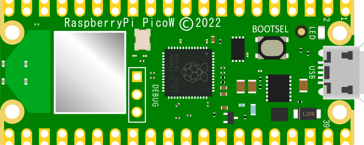
One of the more recent entrants to the world of microcontrollers is the Raspberry Pi Foundation. They have released their RP2040 microcontroller chip which has been distributed on their Raspberry Pi Pico boards.

Computers

Computers are complex devices that are typically comprised of separate microprocessors, memory, bus’s and connectivity for peripheral devices. They are designed to be able to carry out a wide range of tasks and they can vary in size and complexity from large examples which can take up a room to everyday laptop and desktop machines or even our phones.

The feature that they share is that they are collections of discrete circuits that are combined to create a functioning unit. This provides them with greater flexibility so that things like more or less memory can be simply added or a different operating system can be loaded. Like all things, with that capability comes the burden of greater complexity and ultimately cost.

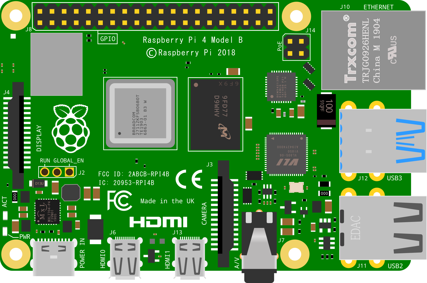
The Raspberry Pi foundation has been manufacturing small, single board computers since 2012 and as such they have come to be a market leader in the supply of small computer boards for computer and electronic hobbyists.

What’s the difference to you?

It’s all very well knowing that there are these different things out there that look kind of similar and act kind of the same, but which have a significant enough difference that people talk about them in quite different ways. What you really want to know is what impact it has on you and the application that you have in mind.

To my way of thinking the application is the first thing to consider when looking at a potential technology direction to go down. Is this a simple application that won’t require a great deal of complexity or change throughout it’s lifetime? In which case a microcontroller could be a good direction. Or, is the application complex, demanding a high level of computing power or frequent updating? In which case a computer could be a better option. There are even cases where either could be viable.

The short answer is that there will always be so many considerations that need to be taken into account that there can’t be a simple guide that can be used to make a decision on whether to use a full blown computer or a microcontroller for a job. The good news is that that piece of information allows us to understand how to approach the problem. In other words, there is unlikely to be a bad decision to make, just different decisions.

That’s where we come full circle here. I’m writing this book so that I can understand the practical use of microcontrollers in a better way. I understand the theory of why they have advantages and disadvantages, but I haven’t really used them in a serious way. I recognise that I need to explore their capabilities and learn more about them so that I can make better decisions about where I could better use a computer over a microcontroller. Hopefully if you’re reading this book, you’re on a similar journey.

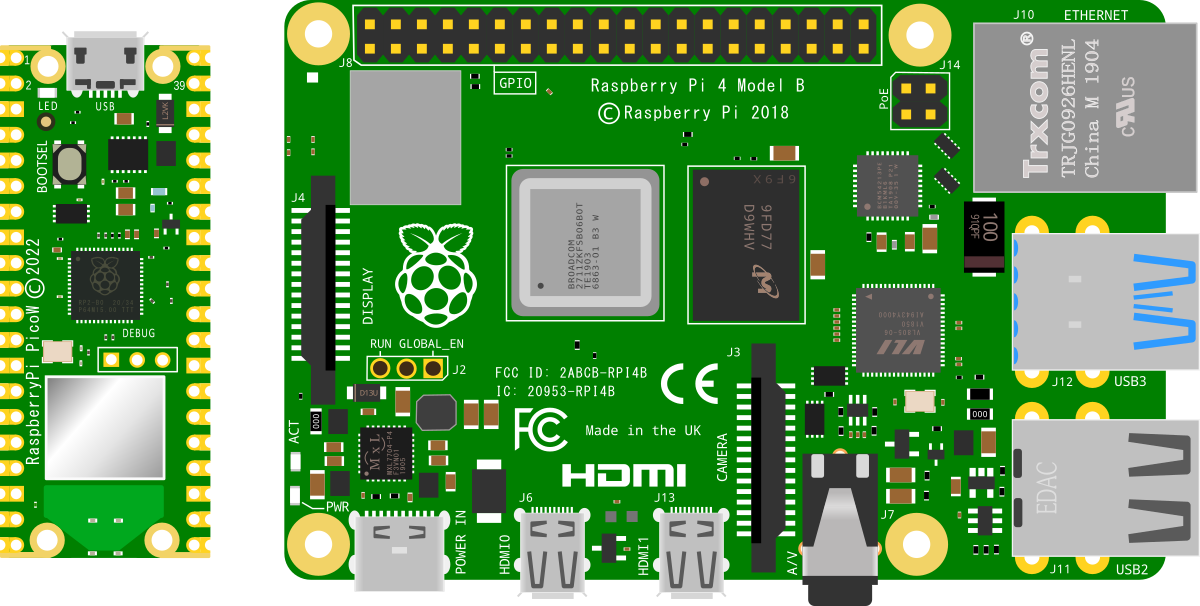
The picture below shows a Raspberry Pi Pico W microcontroller board on the left and a Raspberry Pi 4B computer on the right. They are shown to scale to illustrate their equivalent size, but that’s pretty much where the ease of comparison ends.

The Raspberry Pi Pico

The raspberry Pi Pico is a microcontroller board initially released by the Raspberry Pi Foundation as the ‘Raspberry Pi Pico’ in 2021. It is a board based around the in-house designed microcontroller chip the RP2040.

The RP2040 Microcontroller Chip

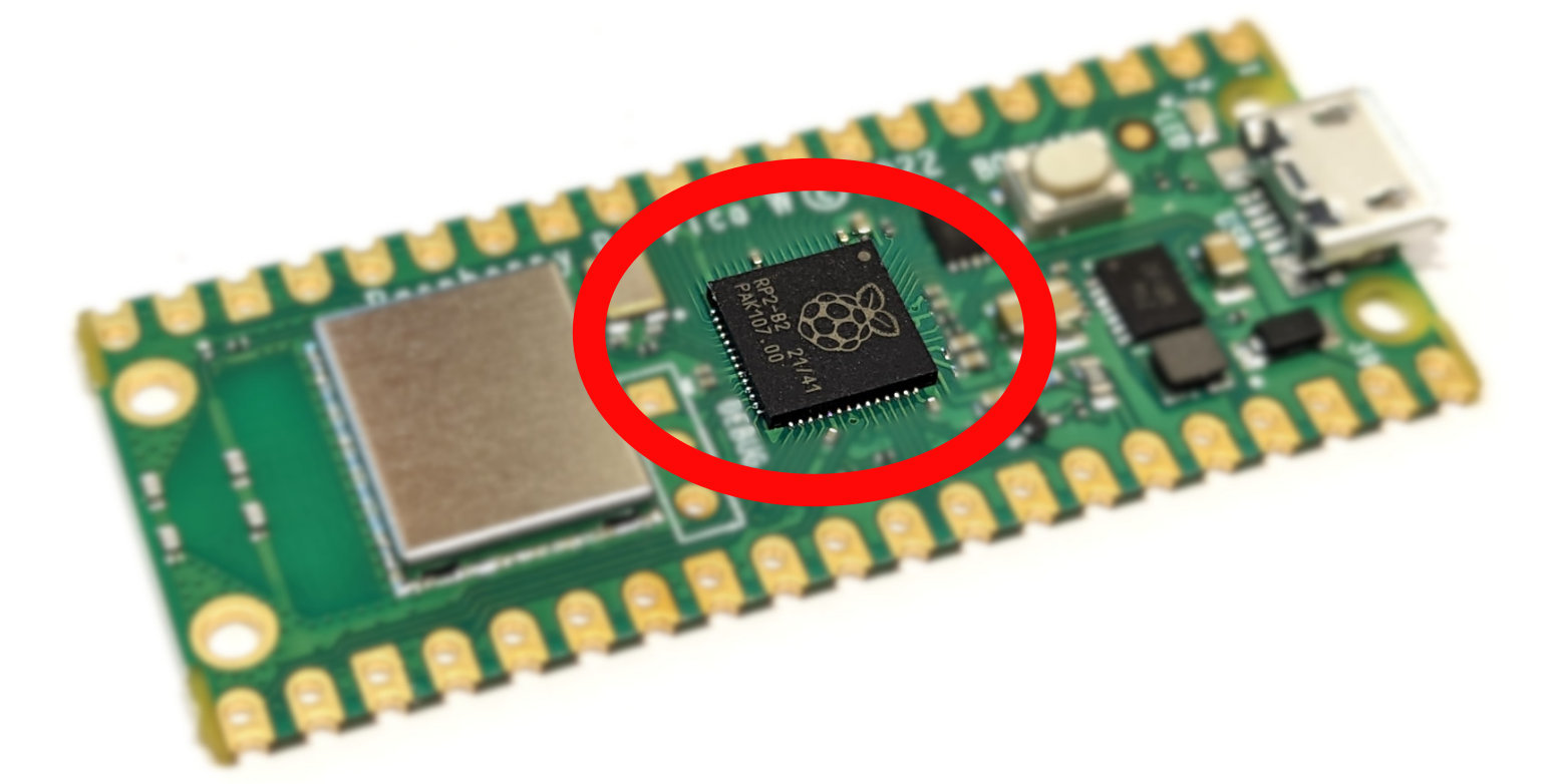
The RP2040 is the first microcontroller released by the Raspberry Pi Foundation. It was designed to deliver high performance, low power consumption and a wide variety of input / output options to provide beginner and hobbyist users with access to a modern and capable option for microcontroller based circuit boards.

It’s key features are;

• A Dual ARM Cortex-M0+ running at 133MHz
• 264kB on-chip SRAM in six independent banks
• Support for up to 16MB of off-chip Flash memory via dedicated QSPI bus
• A Direct Memory Access (DMA) controller
• Fully-connected AMBA High-performance Bus (AHB) crossbar
• Interpolator and integer divider peripherals
• On-chip programmable LDO to generate core voltage
• 2 on-chip Phase Locked Loops (PLLs) to generate USB and core clocks
• 30 General Purpose Input Output (GPIO) pins, 4 of which can be used as analogue inputs

It includes peripheral interconnects in the form of;

• 2 Universal Asynchronous Receiver/Transmitters (UARTs)
• 2 Serial Peripheral Interface (SPI) controllers
• 2 Inter-Integrated Circuit (I2C) controllers
• 16 Pulse-width modulation (PWM) channels
• A USB 1.1 controller with host and device support
• 8 Programmable Input/Output (PIO) state machines (PIO allows you to create additional hardware interfaces, or even new types of interfaces)

The chip can be purchased separately and has been incorporated into a number of different boards manufactured by organisations such as Arduino, Pimoroni, Adafruit, Sparkfun and Lone Dynamics. But arguably the most obvious board manufacturer is the Raspberry Pi Foundation itself.

The Raspberry Pi Pico W Microcontroller Board

At the end of January 2021, the Raspberry Pi Foundation announced the Raspberry Pi Pico as it’s first foray into the world of microcontrollers. The following year the Pico W was released that added (amongst other things) wireless functionality. The description below and pretty much any examples I describe will be using the Pico W.

The board includes the following features;

• 21 mm × 51 mm form factor
• RP2040 microcontroller chip designed by Raspberry Pi in the UK
• 2MB on-board QSPI flash
• 2.4GHz 802.11n wireless LAN option
• Micro USB B port for power and data (and for reprogramming the flash)
• 26 multifunction GPIO pins, including 3 analogue inputs
• 2 × UART, 2 × SPI controllers, 2 × I2C controllers, 16 × PWM channels
• 12-bit 500ksps analogue to digital converter (ADC)
• 1 × USB 1.1 controller and PHY, with host and device support
• 8 × Programmable I/O (PIO) state machines for custom peripheral support
• Supported input power 1.8–5.5V DC and several options for powering the unit from micro USB, external supplies or batteries
• The castellated module allows soldering direct to carrier boards
• Drag-and-drop programming using mass storage over USB
• Low-power sleep and dormant modes
• Accurate on-chip clock
• Temperature sensor
• Accelerated integer and floating-point libraries on-chip

The Pico provides minimum of external circuitry to support the RP2040 chip: flash memory, a crystal, power supplies and decoupling, and USB connector. Four RP2040 I/O are used for internal functions: driving an LED, on-board switch mode power supply (SMPS) power control, and sensing the system voltages. The Pico W has an on-board 2.4GHz wireless interface using 802.11n. The antenna is an onboard antenna formed as a resonant cavity by etching away copper on each layer of the PCB structure. The wireless interface is connected via SPI to the RP2040.

All in all the Raspberry Pi Pico established itself as an immediate realistic option for users of microcontrollers around the World. This in itself is a difficult thing in a dynamic market saturated with options.

Pinout

The Pico W has been designed to make available as much of the RP2040 functionality as possible.

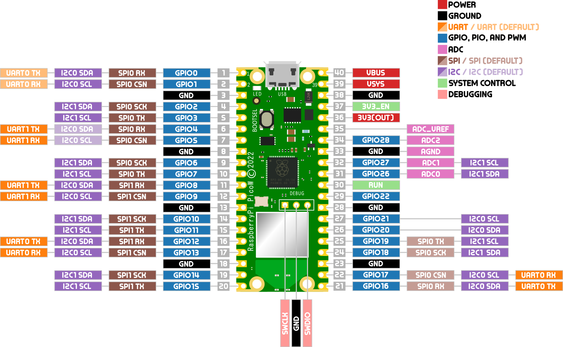
Apart from GPIO and ground pins, there are seven other pins on the main 40-pin interface;

• PIN40 VBUS is the micro-USB input voltage, connected to micro-USB port pin 1. This is nominally 5V.
• PIN39 VSYS is the main system input voltage, which can vary in the allowed range 1.8V to 5.5V.
• PIN37 3V3_EN connects to the on-board SMPS enable pin, and is pulled high (to VSYS) via a 100kΩ resistor. To disable the 3.3V (which also powers off the RP2040), short this pin low.
• PIN36 3V3 is the main 3.3V supply to RP2040 and its I/O, generated by the on-board SMPS. This pin can be used to power external circuitry. It is recommended to keep the load on this pin under 300mA.
• PIN35 ADC_VREF is the ADC power supply (and reference) voltage, and is generated on Pico W by filtering the 3.3V supply. This pin can be used with an external reference if better ADC performance is required.
• PIN33 AGND is the ground reference for GPIO26-29. There is a separate analogue ground plane running under these signals and terminating at this pin. If the ADC is not used or ADC performance is not critical, this pin can be connected to digital ground.
• PIN30 RUN is the RP2040 enable pin, and has an internal (on-chip) pull-up resistor to 3.3V of about ~50kΩ. To reset RP2040, short this pin low.

There is a pdf of the pinout available as an extra when you download the book from Leanpub. I recommend at the least printing out page size copy to have on the bench beside you when working or have it printed to poster size for the wall!

Powering the Pico

There are three main ways we can apply power to the Raspberry Pi Pico. The method used will depend on our application. We can power Raspberry Pi Pico from one of the following;

• The micro USB connector on the device
• The VBUS pin (40)
• The VSYS pin (39).

Powering from the USB connector is by far and away the simplest method, but not always desirable because of limitations of space or supply types.

If we provide a supply to the VBUS pin our Raspberry Pi Pico can take a voltage of between 1.8 and 5.5V, as it has an internal buck-boost regulator (which can regulate the output to a higher or lower voltage than its input). This will internally power VSYS via a Schottky diode, but we must be sure not to connect another power supply to Raspberry Pi Pico’s USB connector at the same time.

The VSYS pin is the main system power supply on Raspberry Pi Pico. From here the Raspberry Pi Pico generates its own 3.3V supply which is used to power RP2040, and also the 3V3 output pin (36). A safe way to add a second power source to Pico W is to feed it into VSYS via another Schottky diode. This will ‘OR’ the two voltages, allowing the higher of either the external voltage (or VBUS) to power VSYS, with the diodes preventing either supply from back-powering the other.

Set up

Setting up our Raspberry Pi Pico for first use is a fairly simple task and I suggest that we should approach it as an exercise in just getting going without too much of an eye to the future.

By that I mean that we should aim to get up and operating with a running program on the Pico. We’ll ignore any plans for connecting peripherals or preparing for installing the device somewhere separate. Our only aim is to get it working and along the way establish how easy it is. We do this so that we can break down any mystique about the process being difficult. This way, if we have a problem, we can work through it with a minimum of complexity.

Our aim therefore is to connect our Raspberry Pi Pico install ‘Thonny’ (which is the programming environment we will use to interact with the Pico) and write a MicroPython program to blink the onboard LED. This is a pretty common example program and should serve to demonstrate that we can get things up and running and from there we can think about more complicated adventures.

Hardware

The hardware requirements are pretty minimal. We will want the following;

• A Raspberry Pi Pico (I will strongly recommend a Pico W and there’s no need to solder any headers onto the board just yet)
• A computer that can run the Thonny Integrated Development Environment (IDE). Pretty much all will be able to.
• A micro USB cable to connect between the Pico and the computer
• A 5V micro USB power source (optional, but cool if we want to demonstrate the Pico running independently from the computer)

Software

The project will guide you through the installation of:

• The Thonny Python IDE
• MicroPython firmware for Raspberry Pi Pico

What is Thonny?

Thonny is a simple Integrated Development Environment (IDE) that is designed to be the logical interface between you (the programmer) and the Pico. This is the application where your can write you code, run it and see the output (and any errors!). IDE’s can be incredibly complex systems that support advanced software development. Thonny is designed for beginners who want to use Python and as such it will more than adequately serve to get us started. It’s also Open Source and as such there are few limitations on getting hold of a copy for use.

Install Thonny

To get hold of the software, go to the official Thonny web site and click on the ‘Download’ button. That will list out the different options that you can choose from depending on the type of computer you are going to be using. Follow the instructions and you will have Thonny installed in a couple of minutes. Open it up.

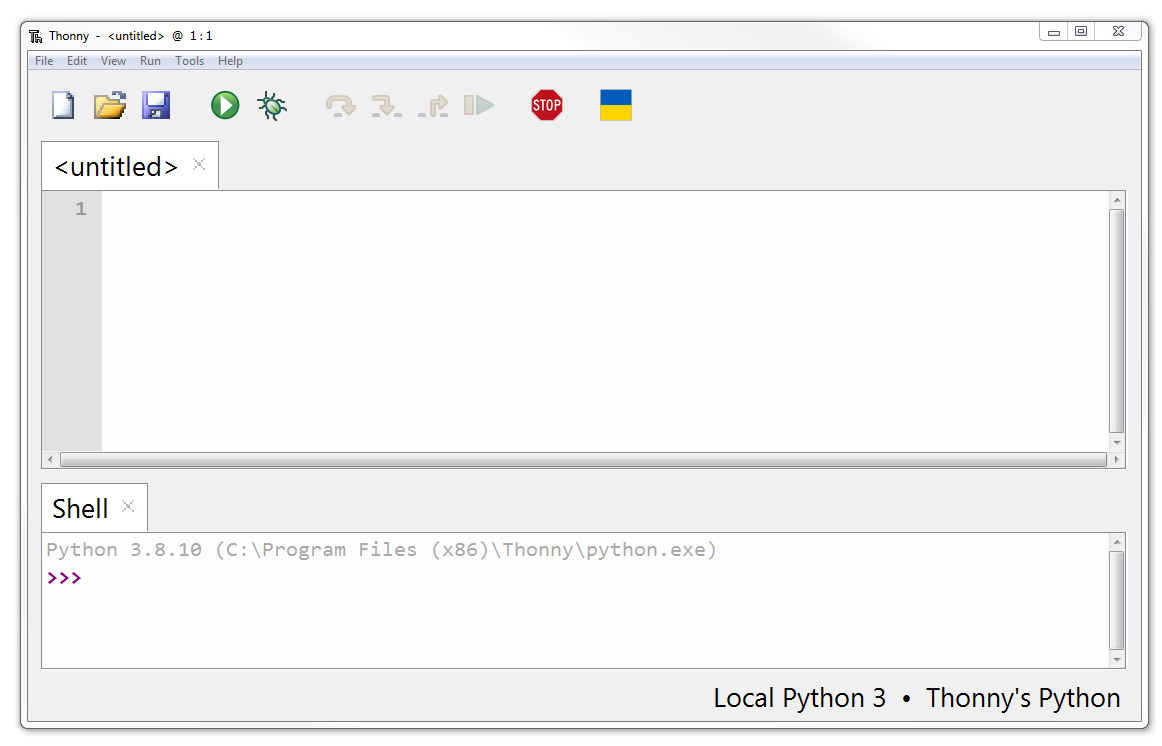
The basic Thonny interface as shown provides us with a code editor in the top section, where we will write all of your code. The bottom half is our ‘Shell’, where we will see any output when we run our code.

In the classic manner of programmers everywhere we can test that things are working correctly by writing a ‘Hello World’ program.

Type the following into the code editor;

print("Hello World")

Then press the ‘Run Script’ button (or press F5).

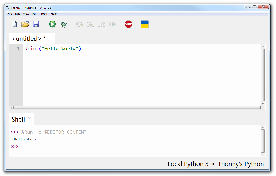
In the shell section of Thonny we should see that the program has run and it has printed out the phrase ‘Hello World’! Congratulations! You’re a programmer! Although perhaps we shouldn’t get ahead of ourselves ;-).

To get a feel for how Thonny can help us out, deliberately break your Hello World program by deleting one of the parenthesis. When we press run again, we should be presented with feedback in the shell that there in an error in the code and it should even provide some indication of where in the code it has occurred. Have a bit of a play and see what changes you can make to both break and expand the code.

What we have been doing above is writing Python code and having it run on our desktop. Now we’re now ready to move on to the next step and connect our Raspberry Pi Pico to Thonny and have the code run on the Pico.

MicroPython

What is MicroPython?

MicroPython is a programming language that is an implementation of the core of Python 3 and includes a small subset of the Python standard library. The simplicity of the Python programming language makes it an excellent choice for beginners who are new to programming and hardware. However, in spite of its name, MicroPython is reasonably full-featured and supports most of Python’s syntax so if you’re comfortable with Python you will be in familiar territory.

MicroPython is optimised for microcontrollers and microcomputers. It is a firmware solution designed to run in constrained environments while allowing a small subset of standard libraries into embedded programming.

MicroPython firmware can run in a footprint of 256 Kilobytes and 16 Kilobytes of RAM. The means we can write clean and simple Python code to control hardware instead of having to use complex low-level languages like C.

So let’s get started!

Connect our Pico

Automatically Installing the Firmware

With Thonny running, connect the Pico to the computer via the cable with the micro USB connector.

In Thonny go to Tools > Options and click on the Interpreter tab. From the interpreter dropdown list select MicroPython (Raspberry Pi Pico).

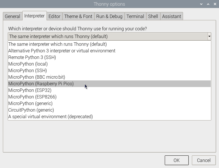
The firmware update dialogue box will open.

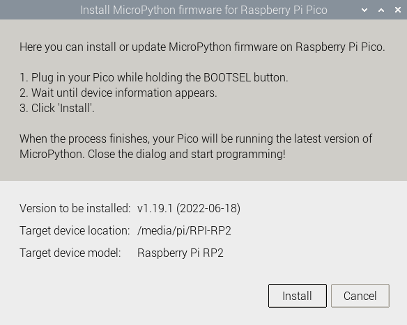
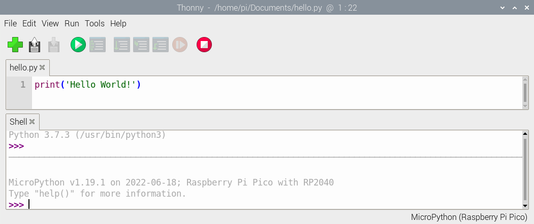
Click on ‘Install’ and once complete we should see the notification in the lower right hand side of the Thonny application indicating that we are running MicroPython on the Raspberry Pi Pico.

Manually Installing the Firmware

Because the Pico W is quite new at time of writing (2022-09-03), we need to be using the latest unstable version of the firmware for it to operate to it’s full potential (at least for the moment).

To load that firmware, download the latest firmware from here.

Then, with the Pico W disconnected from the Pi, press the BOOTSEL button (on the Pico) and plug in the Pico while holding the button down.

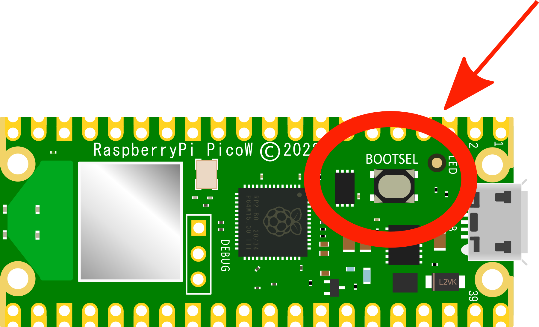
Then release the BOOTSEL button. This will make the Pico act like a mass storage device.

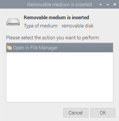
Copy the unstable firmware onto the Pico (just drag it and drop it). Wait for a moment and it will install itself. Once completed, we should see a very modern version of the firmware noted in the Thonny Shell.

Updating Firmware

Because the firmware for the Pico will improve over time, it’s generally a good thing to have it’s firmware updated to the most recent version.

To do this, on the Thonny menu go to Tools >> Options and then select the ‘Interpreter’ tab

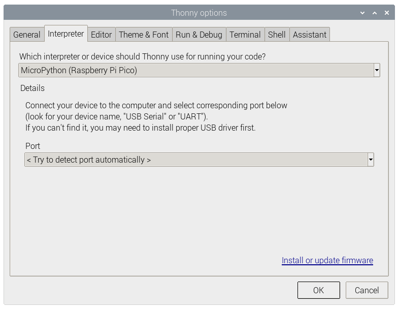
Assuming that we have the correct device selected, select the ‘Install or update firmware’ link.

The firmware update dialogue box will open.

Follow the instructions to plug in the Pico while holding the BOOTSEL button. Once the device information appears (or at the least, the ‘Install’ button isn’t greyed out), click on ‘Install’.

The firmware should be automatically copied from MicroPython.org and installed. I have had an error occur (‘socket.timeout’) in the past, but I just simply clicked on ‘Install’ again and it proceeded without problem.

Close the Options dialog box and press the ‘Stop / Reset’ button on Thonny and we should see our new version of MicroPython displayed at the bottom of the Shell.

Use the Shell

Now we have our Pico connected to our computer and the MicroPython (Raspberry Pi Pico) interpreter in use on Thonny.

This means we can type commands directly into the Shell and have them run on our Pico.

Now we are going to get a little more practical :-).

MicroPython uses hardware-specific modules, such as one called machine, that we can use to program our Pico.

We can create a machine.Pin object to correspond with the on-board LED, which, on the Pico W can be accessed using the reference LED in code.

If you set the value of the LED to 1, it turns on.

Enter the following code in the Thonny editor pane, making sure that we press ‘Enter’ after each line.

from machine import Pin
led = Pin('LED', Pin.OUT)
led.value(1)

If we then press the ‘Run’ icon, a dialog box will come up asking where we want to save our code. This time we’re going to save it to the Pico.

Give the code an appropriate name like led.py and save it. It’s important that we use the file extension ‘py’ as this is what will help the Pico determine how to operate the file.

We should now see the on-board LED light up! Our code has had an effect on the physical world!!!

Edit the code to set led.value to 0 and press the run icon again’ This should turn the LED off.

Turn the LED on and off as many times as you like. Go on. You deserve it :-).

But really… That’s a pretty manual process right? Time to automate!

Blink the on-board LED

It’s time to write a MicroPython program to blink the on-board LED on and off.

Click in the main editor pane of Thonny.

Enter the following code to toggle the LED.

from machine import Pin
import time

led = Pin('LED', Pin.OUT)

while (True):
    led.toggle()
    time.sleep(.2)

Click the Run button to run/save your code. Again, save onto the Pico and a file name like blink.py seems appropriate

We should see the on-board LED turn on and off until we click the Stop button.

Now we’re really starting to cook. But we can do better! Let’s make the led start blinking automatically whenever the Pico is powered on.

Automatically run your program

If you want to run your Raspberry Pi Pico without it being attached to a computer, you need to use a power supply that will conform to the details we laid out earlier for connecting to power. By far and away the easiest method is to simply use a USB power plug.

To automatically run a MicroPython program, all we need to do is save it to the device with the name main.py. Whenever the Pico is powered up, if it sees a file named ‘main.py’ it will automatically start it up.

With our blink.py program in Thonny, go to File >> Save as… Select the Raspberry Pi Pico as the location to save to and name our file main.py.

You can now disconnect our Raspberry Pi Pico from your computer and use a micro USB cable to connect it to a mobile power source, such as a battery pack or a wall-wart.

Once connected, the main.py file should run automatically and our LED will blink!

This is a pretty cool moment because it puts together a bunch of different capabilities that open up a world of new possibilities.

We now know how to program our Raspberry Pi Pico using a language that will allow us to interact with peripherals (all be it an on-board one) and to have that program automatically start whenever our Pico is plugged in.

I think that we’re ready to move on to some tips and tricks :-).

Connectivity

Arguably one of the most important features of a microcontroller is it’s ability to interface with systems outside of itself. Whether that be via a direct connection to the GPIO pins and their many Input / Output (IO) options, via WiFi or even the USB interface. There are a myriad of potential pathways for communication to sensors, other IT devices or directly to us mere humans.

Connecting using Dupont Connectors

Event if you don’t recognise the name, if you’ve played around inside a computer there is a better than even chance that you’ve come across a Dupont connector.

They’re those small black plastic plugs that are used to connect things like the leds or USB connectors to your computers motherboard. They come in a range of different configurations and they are possibly one of the most underused mechanisms available for making ad-hoc connections between your Raspberry Pi Pico and external sensors or small boards. In fact, they can be used with a wide range of different areas and are limited only by the presence of a suitable connection point.

What are Dupont Connectors?

Technically there’s no actual industry term that calls out Dupont connectors. The style people commonly refer to as ‘Dupont’ is a variation of a black, low profile rectangular form with a 2.54mm standard pitch.

Off course the Dupont connector is just one half of a connector pair. The most common mating platform for them is to a header pin. A header pin (or simply a header) is a form of electrical connector. A male pin header consists of one or more rows of metal pins molded into a plastic base, 2.54 mm (0.1 in) apart.

These can be straight, angled, single-in-line, dual-in-line and a myriad of other options.

The Dupont connector slips directly onto a header pin and because they share the same pitch (distance apart of the pins) of 2.54mm they can be similarly ganged together in a myriad of ways.

By far and away the simplest method of utilising this method of connectivity is to purchase bulk lots of the pre-made connectors. These can be male or female and commonly come joined to what is called ‘Rainbow Cable’.

These are incredibly cheap and unless you have a very specific length that is required for a project, they are so easy to use they will quickly become ubiquitous for your project work.

Re-using Connectors

One of the cool things about Dupont connectors is that they can be adjusted by slipping the internal metal connectors out of their casings and placed into new casings. So if you have a set of cables in a three way connector, but the header that you want to connect to doesn’t have the connection points directly beside each other, not problem. Just use a small, flat bladed jewellers screwdriver or similar to gently bend up the plastic flap that is keeping the connector shroud in place. You can then slip the internal wire and connector out of the black plastic housing and place it into three separate single housings. Easy peasy.

Crimping Your Own Dupont Connectors

This is totally do-able and you will find all the materials to carry out the task online. However, as I mentioned earlier, unless you have a specific use for it, it’s probably just easier to utilise the pre-made versions.

However, if you have a need to construct your own connectors, the most important thing to know is that it’s a good idea to practice a few times before doing it for real. It isn’t too hard, but it’s worth having a few tries to get the feel of it. I’m not going to describe the method for constructing your own pins since there are a wealth of different methods and the written word can’t compare to a YouTube video of it being done and that’s not really my bag (maybe one day). I can advise that while there are plenty of tools for doing the job, with a little bit of practice you can get by with a sharp knife / scalpel for stripping the wires (for crying out loud be careful) and a par of needle nosed pliers. Certainly if you’re doing connectors on a regular basis or in an area where there needs to be a high standard of consistency and finish, proper tooling will be essential. But if you’re a hobbyist then why not?

Connectivity via WiFi

The Raspberry Pi Pico W includes an on-board 2.4GHz wireless interface which has the following features:

• WiFi 4 (802.11n), Single-band (2.4 GHz)
• WiFi Protected Access (WPA) 3
• Software enabled Access Point (SoftAP) which supports up to 4 clients

The antenna is a tuned cavity design which is licensed from ABRACON (formerly ProAnt). The wireless interface is connected via a Serial Peripheral Interface (SPI) to the RP2040 microcontroller.

It’s possible to use a standard Pico connected to an ESP8266 or similar to enable WiFi connectivity, but in enabling this I found there was more heartache than I cared to endure. With the release of the Pico W with WiFi built in, this should be the go-to option for connecting to a WiFi network if you’re using a Pico.

Using the network and socket modules

The network module includes functionality in the form of network drivers and routing configuration which is specific to the MicroPython. Drivers for the Pico W hardware is available within this module and it can be used to configure the network interface. Network services are then available for use via the socket module.

Scan for wireless networks

As an example of how the network module provides access consider the following code;

import network
wlan = network.WLAN(network.STA_IF)
wlan.active(True)
print(wlan.scan()) 

When run on a Raspberry Pi Pico W it will enable the network interface, scan for wireless networks and print them out

The import network line imports the network module.

wlan = network.WLAN(network.STA_IF) creates a WLAN network interface object with a client interface type (as opposed to an access point type, which would use network.AP_IF) .

We then activate the network interface with wlan.active(True).

Lastly we print out the results of a scan of available wireless networks with print(wlan.scan()).

The type of output that we would see might look something like the following;

[(b'outside', b"\xb8'\xeb\x81\xb9m", 1, -76, 3, 5), (b'inside', b'l\xb0\xcel\xc0\\
xf4', 6, -37, 5, 9), (b'highway', b'\xdc\xa62*M[', 11, -31, 5, 6)]

Here there are three access points returned with the information apparently separated as ssid, bssid, channel, RSSI, security and hidden. Although, I’ll be honest and say that I know some of those networks and some of those ‘security’ and ‘hidden’ values don’t appear to be correct. More research could be required here.

‘bssid’ is the hardware address of an access point, in binary form, returned as a bytes object. We could use binascii.hexlify() to convert it to ASCII form if we got excited (we will do this in a future project collecting data from temperature sensors).

There are five values for security:

• 0 – open
• 1 – WEP
• 2 – WPA-PSK
• 3 – WPA2-PSK
• 4 – WPA/WPA2-PSK

and two for whether or not the ssid is hidden:

• 0 – visible
• 1 – hidden

Serve a web page

Serving up a web page is well within the Pico W’s capabilities. To do this we will need to active the network interface, connect to a wireless network and then create an http server with a socket connection and then listen for connections and serve up an HTML page.

This is definitely a more complicated process and we are going to make it slightly more so by using two external files to our main.py file. Don’t worry, there’s good reasons for doing so.

Firstly, create a file called secrets.py on the Pico with contents as follows;

secrets = {
    'ssid': 'Replace-with-WiFi-ssid',
    'pw': 'Replace-with-WiFi-Password'
    } 

Edit the file and put the name of the network (ssid) that you’re going to connect to and it’s password in the appropriate places. We are doing this so that when we write our main code, we don’t have to expose things that we would rather not when and if we share our main code.

Next create a file with the contents below and save it as index.html. This will be the web page that we will go to when connecting to the Pico W via the network.

<!DOCTYPE html>
<html>
    <head>
        <title>Pico W</title>
    </head>
    <body>
        <h1>Pico W</h1>
        <p>This is a very simple web page.</p>
        <p>REALLY simple.</p>
    </body>
</html>

Lastly, create the following file on the Pico and call it main.py. This will allow it to automatically start when the Pico is connected to power.

import rp2
import network
import machine
import time
import socket
from secrets import secrets

# Set country to avoid possible errors
rp2.country('NZ')

wlan = network.WLAN(network.STA_IF)
wlan.active(True)

# Load login data from different file for security!
ssid = secrets['ssid']
pw = secrets['pw']

wlan.connect(ssid, pw)

# Wait for connection with 10 second timeout
timeout = 10
while timeout > 0:
    if wlan.status() < 0 or wlan.status() >= 3:
        break
    timeout -= 1
    print('Waiting for connection...')
    time.sleep(1)

wlan_status = wlan.status()

if wlan_status != 3:
    raise RuntimeError('Wi-Fi connection failed')
else:
    print('Connected')
    status = wlan.ifconfig()
    print('ip = ' + status[0])
    
# Function to load in html page    
def get_html(html_name):
    with open(html_name, 'r') as file:
        html = file.read()
    return html

# HTTP server with socket
addr = socket.getaddrinfo('0.0.0.0', 80)[0][-1]

s = socket.socket()
s.setsockopt(socket.SOL_SOCKET, socket.SO_REUSEADDR, 1)
s.bind(addr)
s.listen(1)

print('Listening on', addr)

# Listen for connections
while True:
    cl, addr = s.accept()
    print('Client connected from', addr)
    r = cl.recv(1024)
       
    response = get_html('index.html')
    cl.send('HTTP/1.0 200 OK\r\nContent-type: text/html\r\n\r\n')
    cl.send(response)
    cl.close()

Now run the main.py program. We should see feedback from the shell showing us the connection process and it should include the ip address of the Pico.

Connected
ip = 10.1.1.41
Listening on ('0.0.0.0', 80)

Put the IP address that appears in the shell into a browser that’s on our network and we should see a page giving us the happy news that we have created a web page!

At the same time we should see an indication in the Shell of the connection requests coming in each time we refresh the page.

Connected
ip = 10.1.1.41
Listening on ('0.0.0.0', 80)
Client connected from ('10.1.1.99', 57142)
Client connected from ('10.1.1.99', 57144)
Client connected from ('10.1.1.99', 57145)

There we go. We have just turned our Pico W into a web server! Not only that, but because we have named our program that does it main.py it will operate as soon as we plug in power.

Setting up a static IP address

Enabling network access to the Pico is a really useful thing. This has allowed us to access our device from a separate computer. But when we did it we relied on knowing what the IP address of the Pico was in order to enter that into our browser. The allocation of the address is dynamic and will be dependant on the configuration of our wireless network that is set up by our router. However, we can set up that address so that we know what it is going to be before hand. This is what is called a static IP address.

An Internet Protocol address (IP address) is a numerical label assigned to each device (e.g., computer, printer) participating in a computer network that uses the Internet Protocol for communication.

This description of setting up a static IP address makes the assumption that we have a device running on our network that is assigning IP addresses as required. This sounds complicated, but in fact it is a very common service to be running on even a small home network and most likely on an ADSL modem/router or similar. This function is run as a service called DHCP (Dynamic Host Configuration Protocol). You will need to have access to this device for the purposes of knowing what the allowable ranges are for a static IP address.

The Netmask

A common feature for home modems and routers that run DHCP devices is to allow the user to set up the range of allowable network addresses that can exist on the network. At a higher level we should be able to set a ‘netmask’ which will do the job for us. A netmask looks similar to an IP address, but it allows you to specify the range of addresses for ‘hosts’ (in our case computers) that can be connected to the network.

A very common netmask is 255.255.255.0 which means that the network in question can have any one of the combinations where the final number in the IP address varies. In other words with a netmask of 255.255.255.0, the IP addresses available for devices on the network ‘10.1.1.x’ range from 10.1.1.0 to 10.1.1.255 or in other words any one of 256 unique addresses.

Distinguish Dynamic from Static

The other service that our DHCP server will allow is the setting of a range of addresses that can be assigned dynamically. In other words we will be able to declare that the range from 10.1.1.20 to 10.1.1.255 can be dynamically assigned which leaves 10.1.1.0 to 10.1.1.19 which can be set as static addresses.

Because there are a huge range of different DHCP servers being run on different home networks, I will have to leave you with those descriptions and the advice to consult your devices manual to help you find an IP address that can be assigned as a static address. Make sure that the assigned number has not already been taken by another device. In a perfect world we would hold a list of any devices which have static addresses so that our Pico’s address does not clash with any other device.

For the sake of this exercise we will assume that the address 10.1.1.110 is available.

Default Gateway

We will also need to find out what the default gateway is for our network. A default gateway is an IP address that a device (typically a router) will use when it is asked to go to an address that it doesn’t immediately recognise. This would most commonly occur when a computer on a home network wants to contact a computer on the Internet. The default gateway is therefore typically the address of the modem / router on your home network.

We can check to find out what our default gateway is from Windows by going to the command prompt (Start > Accessories > Command Prompt) and typing;

This should present a range of information including a section that looks a little like the following;

Ethernet adapter Local Area Connection:

  IPv4 Address. . . . . . . . . . . : 10.1.1.15
  Subnet Mask . . . . . . . . . . . : 255.255.255.0
  Default Gateway . . . . . . . . . : 10.1.1.1

The default router gateway is therefore ‘10.1.1.1’.

With all that information we are now ready to configure our static IP address.

Configure the static IP

Our network module and our WLAN class include an ifconfig method that uses all our gathered information’. We will need to declare it in the format wlan.ifconfig([(ip, subnet, gateway, dns)]).

When called with no arguments, this method returns a 4-tuple with the above information. To set the above values, pass a 4-tuple with the required information. For example:

wlan.ifconfig(('10.1.1.110', '255.255.255.0', '10.1.1.1', '8.8.8.8'))

Where 8.8.8.8 is a suitable DNS server.

To include it in the example of server our web server, we would slot it into the section where we are configuring the wlan settings;

wlan = network.WLAN(network.STA_IF)
wlan.active(True)
wlan.connect(ssid, password)
wlan.ifconfig(('10.1.1.110','255.255.255.0','10.1.1.1','8.8.8.8'))

Give it a try!

General Purpose Input / Output (GPIO)

The Raspberry Pi Pico has 26 multi-function General Purpose Input / Output (GPIO) pins available for connecting to external devices. 23 of them are digital only pins and three are also capable of acting as software selectable Analogue to Digital Converters (ADC). The voltage for the digital output is made available from the 3.3V rail.

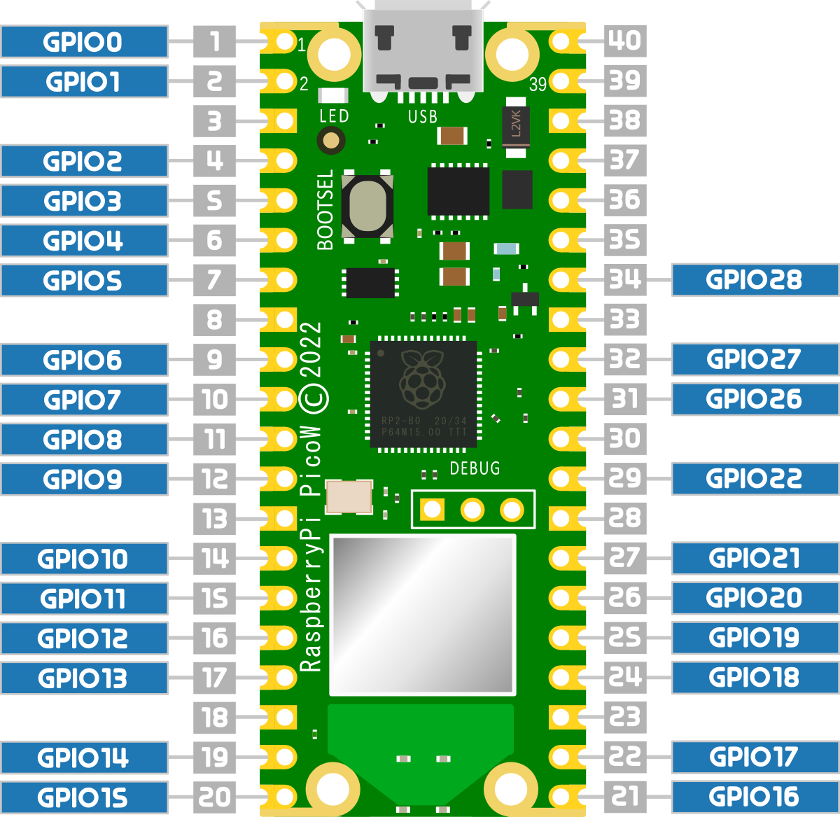
The observant reader will notice that the numbers above seem a little out of whack with the numbered pins on the Pico pinout. Here they go from zero to 28, but numbers 23, 24 and 25 are missing. Hence 26 total are exposed to the header pins.

The three missing pins (23, 24 and 25) in the sequence along with GPIO29 are used for internal board functions;

On the original Pico those functions are;

• GPIO23 OP wireless power on signal
• GPIO24 OP/IP wireless SPI data/IRQ
• GPIO25 OP wireless SPI CS when high also enables GPIO29 ADC pin to read VSYS
• GPIO29 OP/IP wireless SPI CLK/ADC mode (ADC3) to measure VSYS/3

And on the Pico W the functions are;

• GPIO23 OP Controls the on-board SMPS Power Save pin
• GPIO24 IP VBUS sense high if VBUS is present, else low
• GPIO25 OP Connected to user LED
• GPIO29 IP Used in ADC mode (ADC3) to measure VSYS/3

The exposed GPIO pins can be utilised as inputs or outputs for a range of different protocols and functions. These are in turn configured and enabled in software and can include;

• Serial Peripheral Interface (SPI): is a synchronous serial communication interface specification used for short-distance communication.
• Universal Asynchronous Receiver-Transmitter (UART): is a function for asynchronous serial communication where the data format and transmission speeds are configurable.
• Inter-Integrated Circuit (I2C): is a commonly used 2-wire interface that can be used to connect devices for low speed data transfer using clock and data wires.
• Pulse width modulation (PWM): is a method of reducing the average power delivered by an electrical signal, by effectively chopping it up into discrete parts.
• Analogue to Digital Converter (ADC): takes an analogue signal, such as a variable voltage level, into a digital signal.

Pull-up and Pull-down Resistors

When setting up a GPIO pin as an input, it is important to provide a stable state at the pin to enable a reliable reading. It’s easy to simply think that this has to occur when an important event occurs like sensing a high level from a switch or when triggering from a pulse, but the reality is that a GPIO pin is looking for a reading of one of two states. We can call them a range of different things like;

• High and low
• On and off
• 3.3V and ground
• 1 and 0

Whatever we call them the important fact is that the signal level can be distinguished between two different states.

This means that when we want to register when a high voltage occurs on a pin, first we need to know what the low voltage is. And visa versa. If we are looking to try and read when a pin drops to ground, first the pin needs to be able to recognise the 3.3V is the high point.

We accomplish this feat of knowing our reference points by using pull-up and pull-down resistors on our Pico.

What does pull-up and pull-down actually mean?

The answer to the question is kind of in the name, but that doesn’t necessarily make it obvious. It’s also really useful to frame the question by using an example, and in our case (since this is being written for a book about the Raspberry Pi Pico) we can use a GPIO pin on the Pico as our case study.

We like to talk about our ability to read either a high or low signal on our GPIO inputs, but the reality is that there are three states that our voltage measuring effort could result in. A low state that will typically be ground or 0V, a high state that will typically be about 3.3V, and a mysterious third state which is ‘floating’.

We can illustrate this by attempting to measure the voltages on our Pico.

The low state

Using a meter to measure the voltage on our Pico, we can first ensure that there is a common reference point set by connecting our negative probe to a ground pin (here pin 23) and we can then measure the amount of voltage or potential difference is present between that ground pin and another (pin 33 shown here).

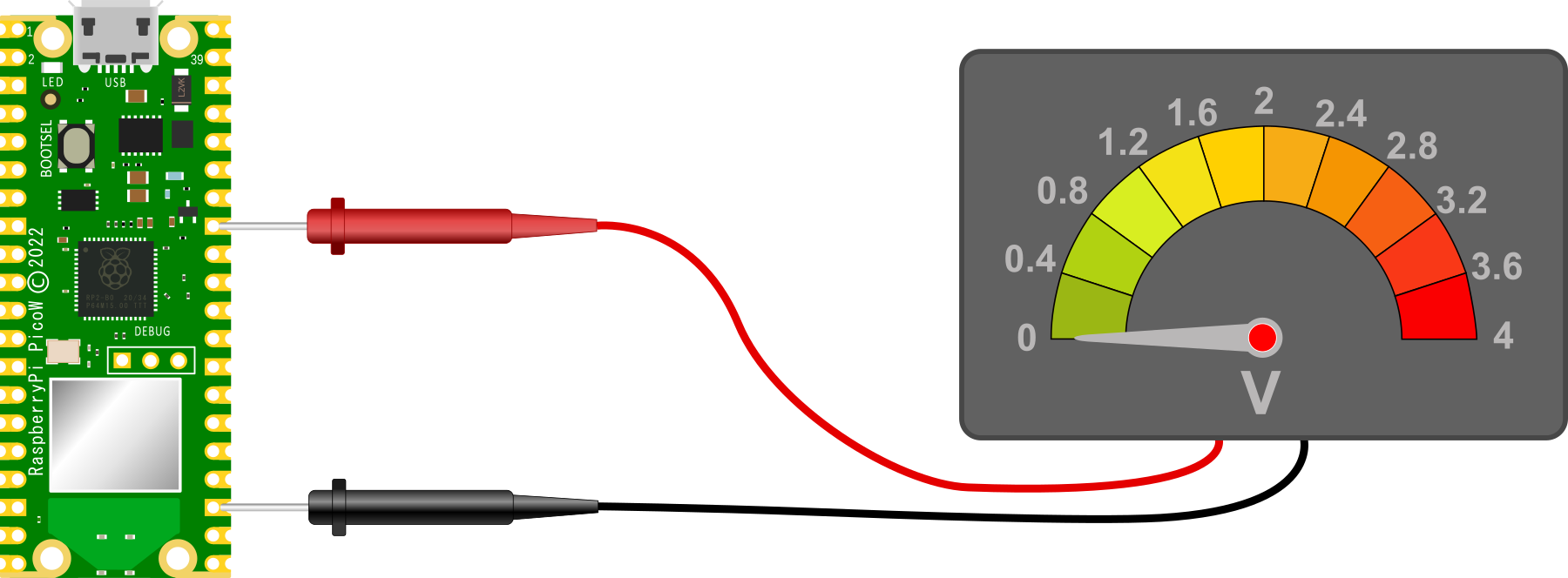
Unsurprisingly, we should read 0V. This is because the two ground pins are connected together on the circuit board and represent exactly the same voltage. Therefore the difference between them is 0V.

The high state

With our voltmeter measuring the difference between our common reference point of ground and the 3V3(OUT) pin (36), we are naturally going to read a voltage of 3.3V.

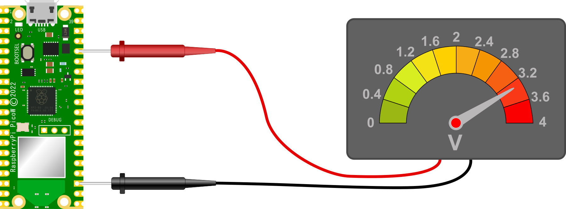
Again unsurprisingly we see 3.3V because there is a potential difference between the ground pin (23) and the 3V3(OUT) pin (36) of 3.3V

The floating state

And now to our ‘floating’ state. with our red lead removed from our Pico and floating in mid air, we have an uncertain reading on our voltmeter

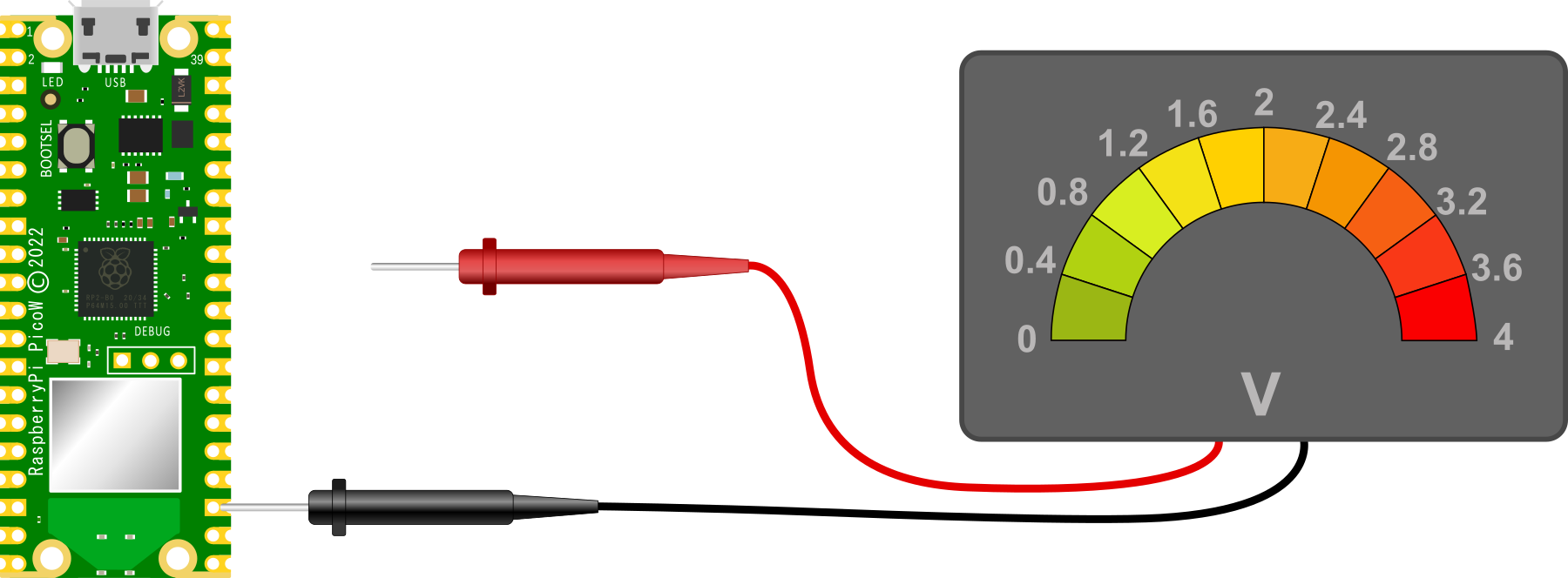
This situation is a bit like Schroedinger’s cat in the quantum state analogy. We can’t confirm if it’s alive or dead, so it’s both simultaneously. Except in this case, the reading is uncertain and we cannot state what it will be since there the meter is not fully connected to the circuit.

This floating state is the initial configuration of our GPIO pins on the Raspberry Pi Pico. Each one of them is essentially disconnected and as a result we can’t expect to read a steady voltage off them.

Pulling our pin

So to set our GPIO pins to a state where they have a reliable reference voltage we need to ‘pull’ the voltage either up or down so that in a resting state they read high or low.

A pull-up or pull-down resistor is connected so that the GPIO pin is connected to either ground or 3.3V via a resistance.

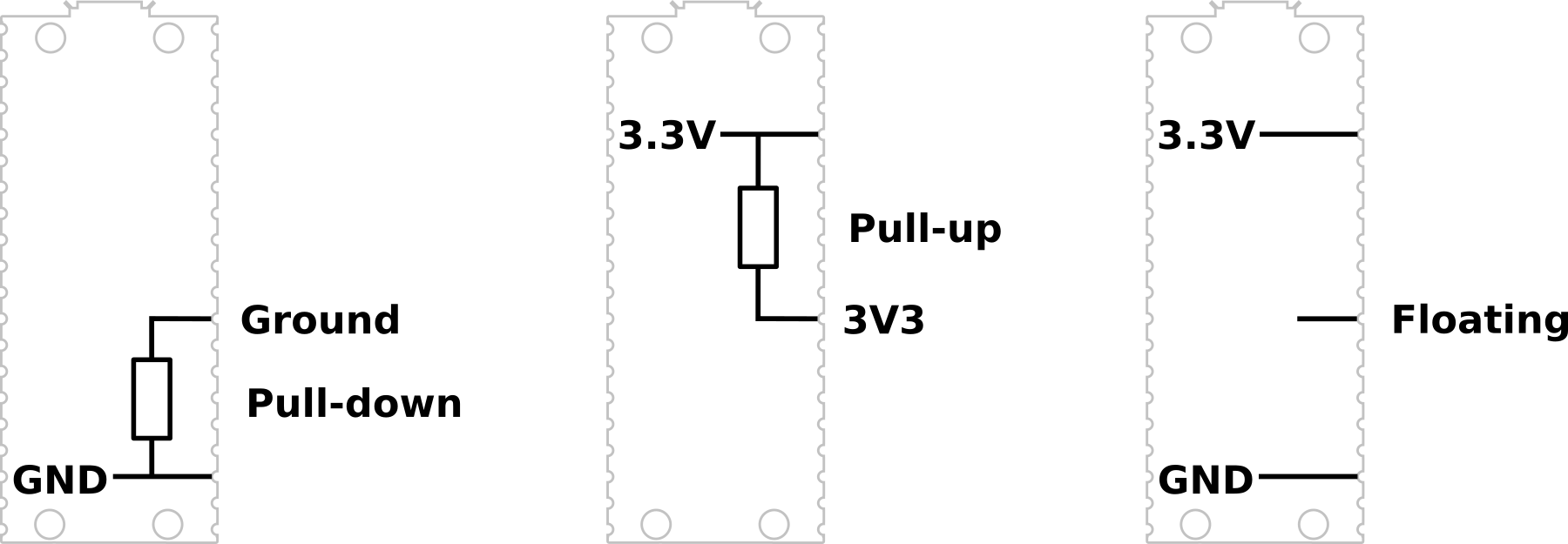
In some circuits this might be necessary to implement using discrete components, but the RP2040 microcontroller can configure a GPIO pin as either pull-up or pull-down internally and we just need to instruct it to do so via software. The resistance value in the pico is specified as being between a minimum of 50kΩ and a maximum of 80kΩ.

For example, in the PIR section of this book we set up our GPIO pin as an input and then we configured the pin as pull-down via the following code;

from machine import Pin

pir = Pin(22, Pin.IN, Pin.PULL_DOWN)

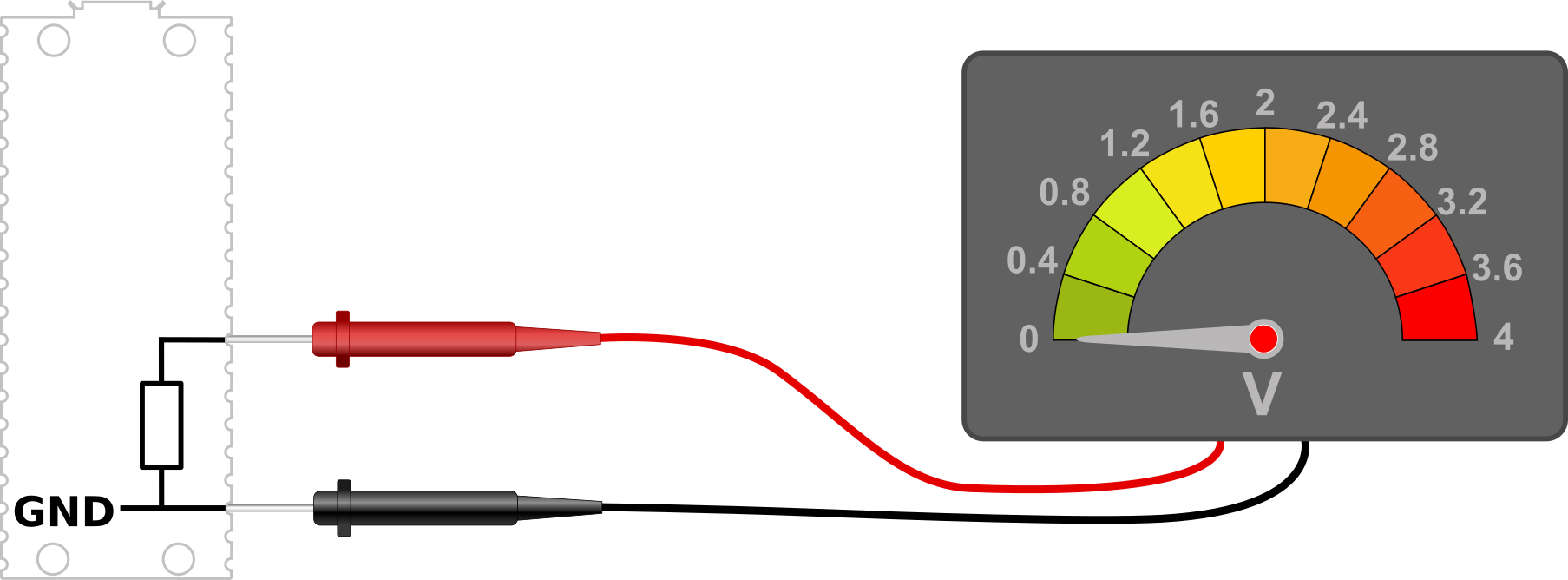
We can test our thinking by considering reading the voltage at our nominal GPIO pin with the Pin.PULL_DOWN configuration set. That will read 0V.

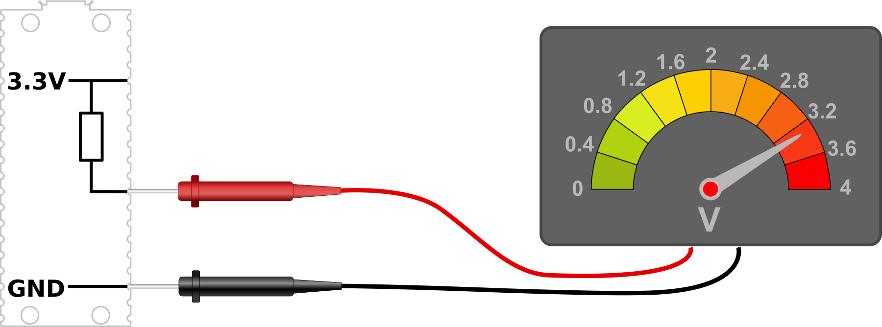
Conversely with the GPIO pin set to Pin.PULL_UP we will have the following circuit where we will read a voltage of 3.3V.

Once we have set the GPIO pin to its default state of high or low we can then go about the job of varying that pin to the alternate state via whatever input we choose. For example via a PIR or a common switch.

Inter-Integrated Circuit (I2C)

The Raspberry Pi Pico includes support to the I2C communications protocol through two I2C controllers which combined service a total of 12 separate connection pair options.

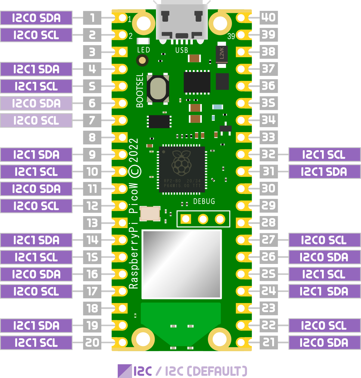
Right from the outset, this does not mean that we can hook up multiple devices (or string of devices) to multiple connection points that use the same controller. One device or string of devices per controller only. That means that we are limited to a total of 127 daisy chained devices per controller. That should be enough for a start :-).

I2C (Inter-Integrated Circuit) is a serial communication protocol that allows devices to communicate with each other over a shared bus. It was developed in the 1980s by Philips Semiconductors as a way to reduce the number of wires needed to connect devices, and has become widely used in a variety of applications.

I2C uses a two-wire interface, consisting of a serial data line (SDA) and a serial clock line (SCL). Devices that use I2C are called ‘slaves’, and they are connected to a ‘master’ device (usually a microcontroller or processor) through these two wires. The master device controls the communication by generating the clock signal and sending/receiving data on the SDA line.

I2C is a very useful protocol because it allows multiple devices to communicate with a single microcontroller or processor using just two wires, making it well suited for use in embedded systems and other applications where space and resources are limited. It is also relatively simple to implement, making it a popular choice for many applications.

How does I2C work?

The master device controls the communication by generating the clock signal and sending/receiving data on the SDA line. The slave devices are connected to the master device through the SDA and SCL lines, and they respond to the commands and requests of the master device.

Here is a brief overview of how I2C works:

• The master device starts the communication by pulling the SDA line low while the SCL line is high and then pulling the SCL line low as well, indicating the start of a new data transfer.

• The master device then sends a 7-bit slave address followed by a read/write bit, indicating whether it wants to read data from or write data to the slave device.

• If the slave device recognizes its own address, it sends an acknowledgement (ACK) by pulling the SDA line low. If the slave device does not recognize its own address, it does not send an ACK and the communication ends.

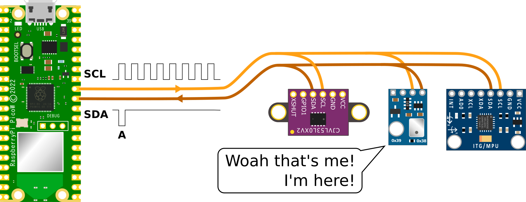
• If the master device wants to write data to the slave device, it sends the data byte by byte, followed by an ACK from the slave device after each byte. If the master device wants to read data from the slave device, it sends a request for data and the slave device responds by sending a byte of data followed by an ACK from the master device.

• The communication ends when the master device sends a stop condition by pulling the SDA line high while the SCL line is high.

Finding and I2C devices connected to the Raspberry Pi Pico

On the Raspberry Pi Pico, I2C is implemented using a hardware peripheral called the I2C controller, which is part of the Pico’s RP2040 microcontroller. The I2C controller is responsible for generating the clock signal and managing the communication between the Pico and I2C slave devices.

To use I2C on the Raspberry Pi Pico, you will need to import the machine module and use its I2C class.

The following code that demonstrates how to scan for I2C slave devices on the Raspberry Pi Pico and print the addresses of the detected devices.

import machine

# Create an I2C object with the specified SDA and SCL pins
i2c = machine.I2C(sda=machine.Pin(22), scl=machine.Pin(23))

# Scan for slave devices on the I2C bus
devices = i2c.scan()

# Print the addresses of the detected devices
print(devices)

This code creates an I2C object using the SDA and SCL pins 22 and 23, respectively, and uses the scan() method to detect slave devices on the I2C bus. It then prints the addresses of the detected devices.

Serial Peripheral Interface (SPI)

What is the Serial Peripheral Interface protocol?

A Serial Peripheral Interface (SPI) is a type of serial communication protocol used to transfer data to devices such as sensors, displays, and other peripherals. It is a full-duplex, synchronous communication protocol that uses four wires to communicate;

1. A clock signal (SCK)
2. A data out signal (Master Out Slave In, or MOSI - connected to the Pico SPI TX line)
3. A data in signal (Master In Slave Out, or MISO - connected to the Pico SPI RX line), and
4. A chip select signal (SS or CS or CSN).

How does SPI work?

In an SPI system, there is one device that is designated as the master, and one or more devices that are designated as slaves. The master device generates the clock signal and controls the communication by asserting the chip select signal for the slave device it wants to communicate with. The slave device responds by sending or receiving data over the MISO and MOSI lines.

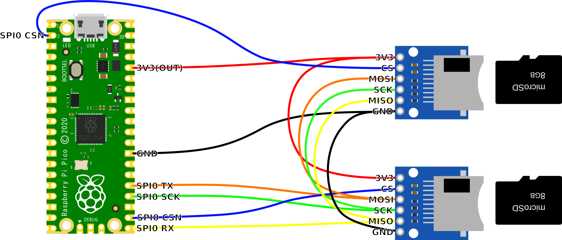
A simplified description of how an SPI communication cycle works is as follows;

• The master asserts the chip select signal for the slave device it wants to communicate with.
• The master sends a command or data over the MOSI line to the slave.
• The slave receives the data and sends a response over the MISO line to the master.
• The master receives the response and de-asserts the chip select signal, signalling the end of the communication cycle.

This process can be repeated multiple times to transfer multiple bytes of data. The clock signal determines the speed of communication, with higher clock speeds allowing for faster data transfer.

SPI is similar in function to I2C (Inter-Integrated Circuit), but where SPI is at a disadvantage in terms of the number of wires used and a more limited number of connected devices, it has the advantage of much higher data transfer speeds.

How is SPI implemented on the Raspberry Pi Pico?

The Raspberry Pi Pico has two built-in SPI controllers courtesy of the two SPI channels on the RP2040. There are a choice of pins that may be used for the SPI signals, but you can only define one set per channel. As well as this, each device will need it’s own dedicated chip select connection.

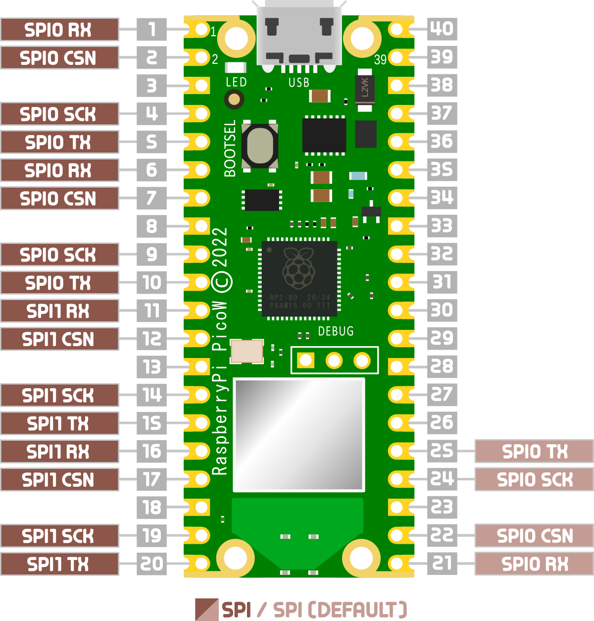
Looking at the pinout for the Pico we can see that there are three chip select connectors for SPI0 and two for SPI1.

In fairness, it is possible to use the process known as ‘bit-banging’ to simulate an SPI interface on any GPIO pin, but we will need to take into account a slower speed and increased susceptibility to noise.

Reed Switches with the Raspberry Pi Pico

Reading the state of a switch is a pretty basic function for a microcontroller, but it’s an action that is worth understanding and we can add a little bit of spice to it by using a switch that is commonly used in security systems and to detect the state of items that need to determine whether they are open or closed (fridges, laptops, washing machines).

What is a Reed Switch?

Reed switches are type of switch that are actuated via the presence of a magnetic field. They are typically constructed of two thin, flexible, ferromagnetic metal wires or blades (these are the reason that the switch is called a ‘reed’ switch). The blades are positioned slightly apart in a sealed glass tube. When it is placed in close enough proximity to a magnet that has enough strength to trigger the required level of actuation, the metal reed bends and the switch is made.

While this is a pretty cool type of switch, it’s function is the same as a wide range of other switch types from a standard push-button to a lever type to simply pressing two wires together. Basically it’s a way of connecting an electrical circuit.

The Magnetic Reed Switch

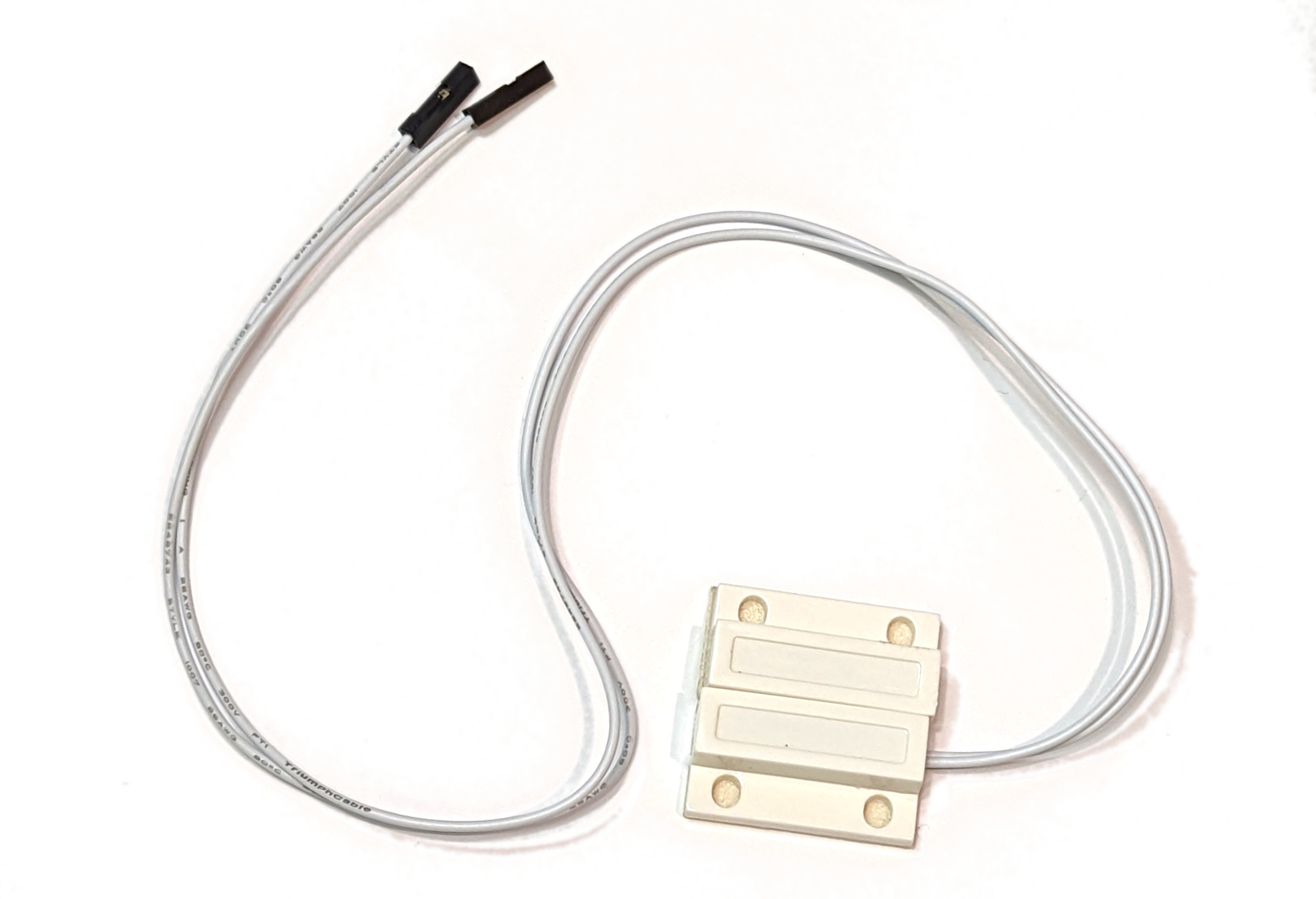
Our reed switch comes as the switch proper which is encased in a plastic mount with flying leads coming off it. In the picture that follows I have crimped two Dupont connectors onto the end of the leads for ease of connecting to the Pico. There is also a separate magnetic activator which, when moved close to the switch will enable it. I.e. we can imagine the portion with the leads mounted on a window frame and the magnetic activator portion mounted on the window proper.

How do we read a switch?

A switch is one of the simplest sensors to read. Once the input is configured in software, the two leads of the switch can be connected to the appropriate pins and we’re good to go. When the switch is made (or un-made) the state of the input changes and the Pico can read the input.

Pull-up or pull-down?

The main driver for the connection type is understanding what the switch is going to be switching. This might be dictated if you’re using a particular type of sensor, but for standard switch, we have two choices depending on whether we want to connect our switch to the 3.3V connection or the ground (the other end of the switch will be going to the GPIO pin).

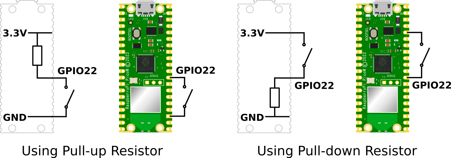
For a deeper explanation of how pull-up and pull-down resistors are selected and implemented in a circuit or a Pico, check out the section on pull-up and pull-down setting of GPIO pins earlier in the book.

If we’re connecting a simple switch, either method is as good as the other. However, I would normally opt for the pull-up option on the basis that it is easier to find a spare ground connector than it is to try and connect to the sole 3.3V pin.

With that in mind, the example that follows will configure our GPIO pin with a pull-up resistor and we will connect our reed switch between a ground pin (we’ll go for pin 23) and GPIO 22 (pin 29).

Connecting up the switch to the Pico

Because we are opting to use an internal pull-up resistor, we will connect our switch between a ground pin (pin 23 in this case) and GPIO22 (pin 29).

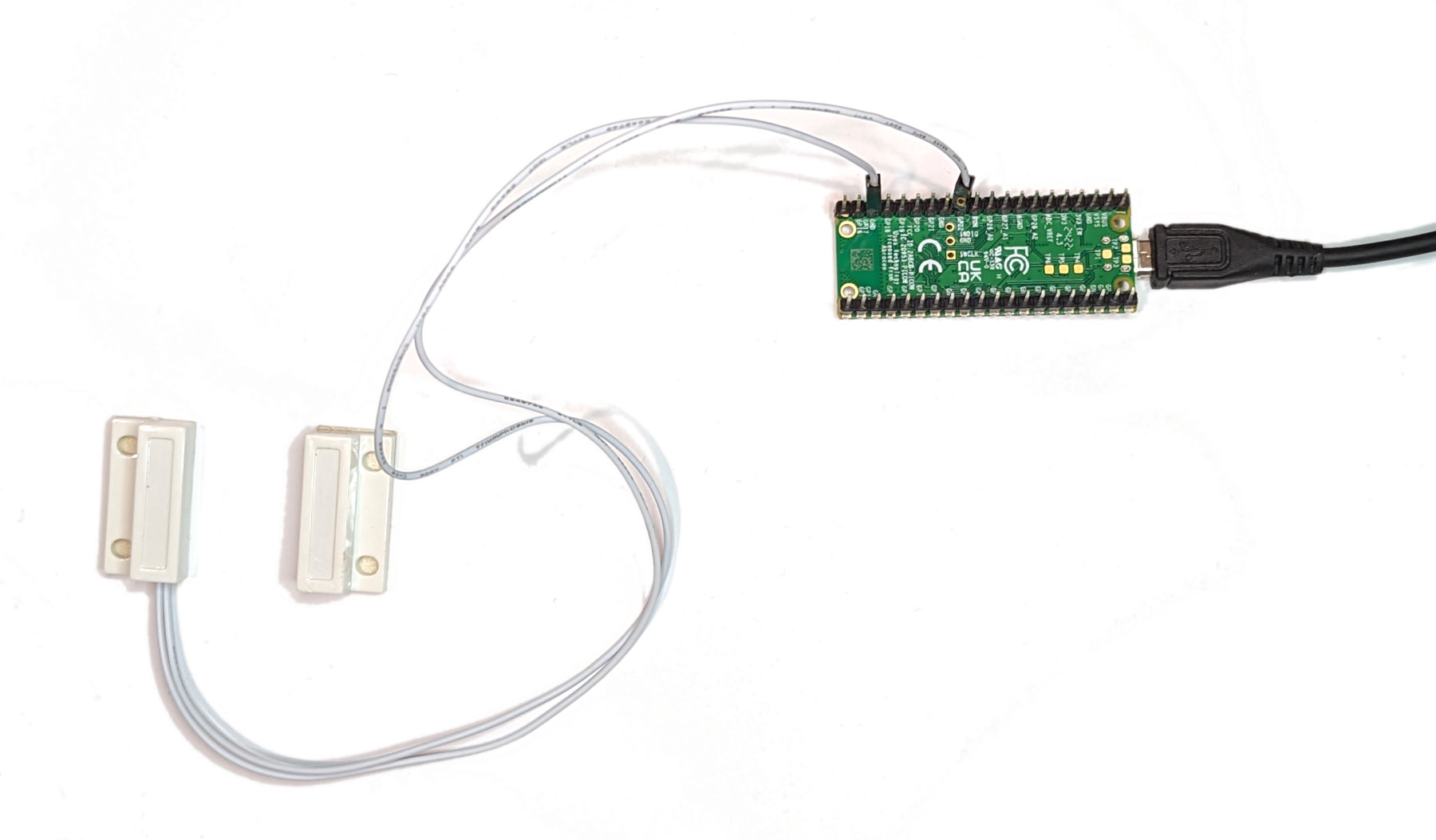
It makes no difference which way round the leads are connected.

Code

The code below will designate the GPIO pin to be used as our input (GPIO22) and set it to a default high state with a pull up resistor.

switch = Pin(22, Pin.IN, Pin.PULL_UP)

We will also need to set the GPIO pin to be an input (seen above as Pin.IN). Once set to input, the GPIO line is high impedance so it won’t draw very much current, no matter what we connect it to.

Our method to read the state of the switch is via the switch.value() parameter. Normally our GPIO pin will be high since our switch is a ‘normally open’ switch, but once the magnet is moved close to the main body of the reed switch, the mechanism closes, the switch is made and the GPIO pin is then connected to ground and reads 0V.

Just to make things interesting, it increments a counter and loops repeatedly incrementing when the switch is closed.

import time
from machine import Pin

switch = Pin(22, Pin.IN, Pin.PULL_UP)
count = 0

time.sleep(1)
print('Ready to switch!')

while True:
     if switch.value() != 1:
          count = count + 1
          print('Switch closed ', count)
          time.sleep(4)
     time.sleep(1)

Controlling a Servo from the Raspberry Pi Pico

What is a Servo Motor?

Servo motors are types of motors that have been designed to rotate precisely in response to control signals. They are commonly used in applications such as robotics and remote control vehicles to provide a specific angle or distance of movement.

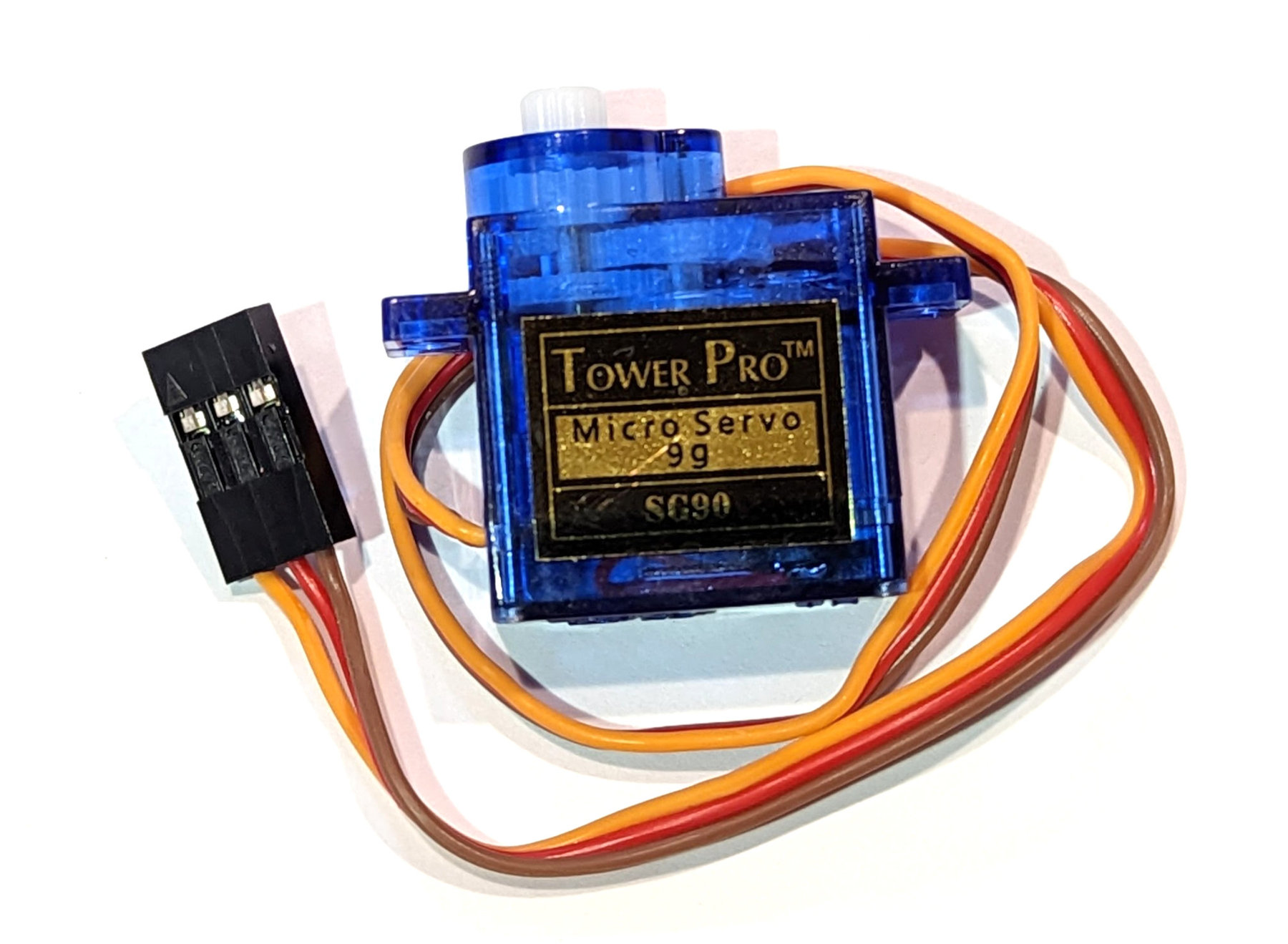
They are rated in kg/cm (kilogram per centimetre) which translates as how much weight the servo motor can lift at a particular distance. For example: A 5kg/cm servo motor should be able to lift 5kg when its load is suspended 1cm from the motors shaft, the greater the distance of the weight from the shaft, the less the weight lifting capacity.

How does a Servo Motor Work?

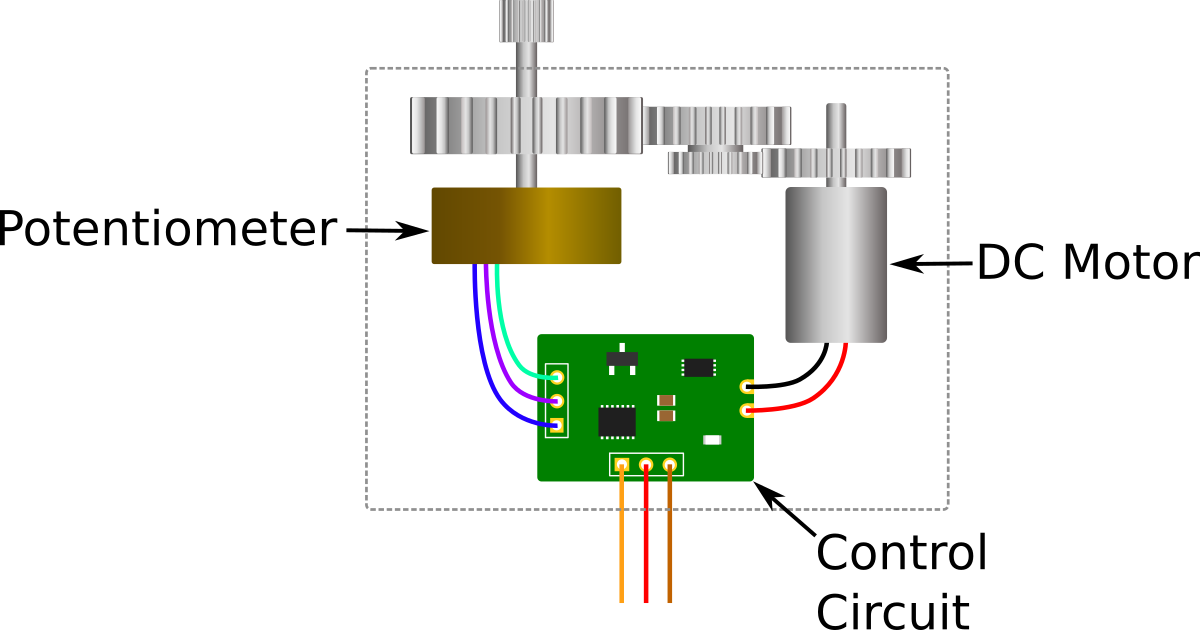
A servo motor can use an AC or DC motor as its driving force and this is one of the many different methods of describing them. In a very simple example, a DC servo motor will employ a simple DC motor, gears, a potentiometer and a control circuit. In response to an input signal on the control circuit, the motor and the gears rotate and the potentiometer’s resistance changes. This provides feedback to the control circuit which regulates how much movement there is and in which direction.

How is a Servo Motor Controlled?

A typical servo motor will have three wires. Two for power supply (positive and ground) and one for the controlling signal.

The controlling signal is a pulse of variable width, and thus the controlling mechanism is named Pulse Width Modulation (PWM). A pulse is sent every 20 milliseconds. The width of the pulses determine the position of the shaft. So, a pulse width of 1ms will move the shaft anticlockwise by 90°, a pulse of 1.5ms will move the shaft to a ‘neutral’ position at 0° and a pulse of 2ms will move the shaft clockwise by +90°.

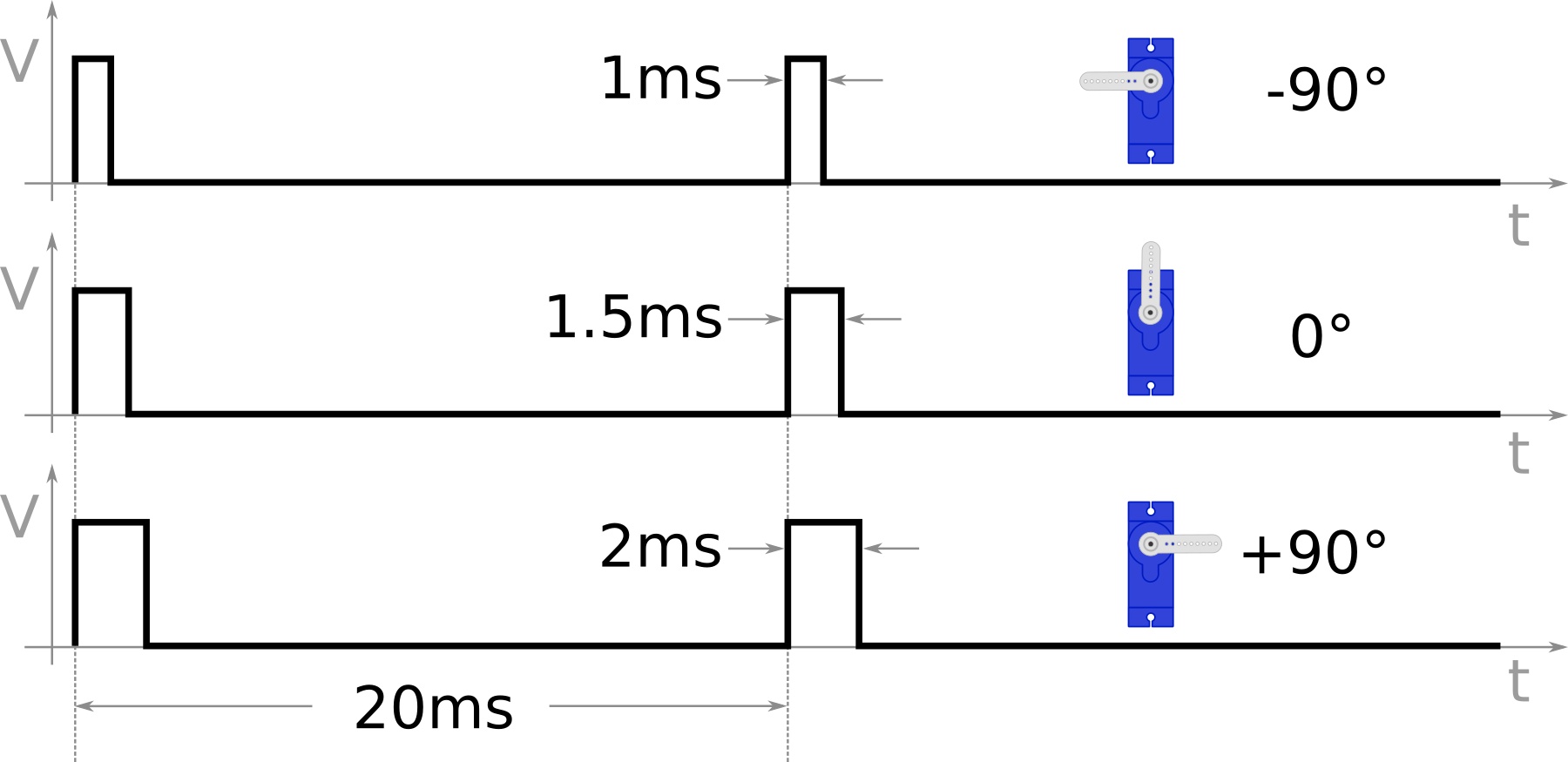
A typical servo motor will only turn 90° in either direction and will have a mechanical stop to prevent further movement.

When a servos is commanded to move, it will move to the position specified by the pulse width and hold that position. The maximum amount of force the servo can exert is called the torque rating of the servo. As an example of this force, when we are running our code below and the servo motor is connected and powered on, try (gently) to move the arm. There should be a reasonable resistance. If you disconnect the power the servo can be moved relatively easily.

Connecting Everything Up to the Pico

The example shown here uses a SG90 micro servo. It is a very small and inexpensive servo that can rotate approximately 180 degrees (90 in each direction). These are immensely popular for simple jobs or learning about the principles of servos. It typically comes with 3 arms and fixing hardware. Its operating voltage is from 4.8V to 6V and at 4.8V it has a torque of 2.0kg/cm and will move through 60° in 0.1s.

We will connect;

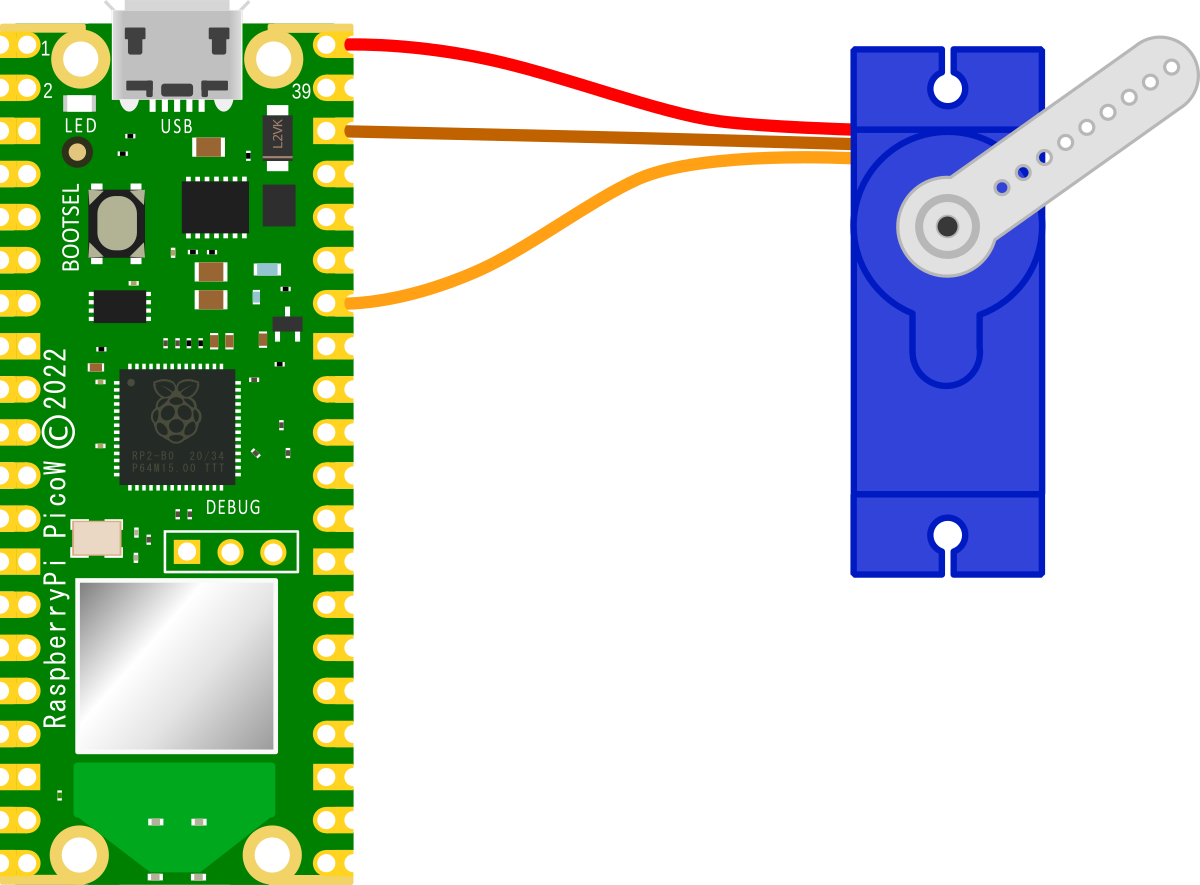
• The red wire (VCC) to the VBUS pin (40) on the Pico (this makes the assumption that we are powering our Pico from a source connected to the micro USB connector with the standard 5V applied)
• The brown wire (Ground) to the ground pin (38) on the Pico
• The orange wire (the PWM signal) to GP28 (pin 34) on the Pico

All of the GP pins on the Pico can be used for pulse width modulation control. This is because the RP2040 has 8 identical PWM ‘slices’, each with two output channels (A/B), where the B pin can also be used as an input for frequency / duty cycle measurement. This means that each slice can drive two PWM output signals, or measure the frequency / duty cycle of an input signal. This provides a total of up to 16 controllable PWM outputs.

Since all of the GP pins can be driven by the PWM block, it’s just a matter of selecting which one you would like to use.

I selected GP28 (pin 34) for no better reason than it made drawing the connection diagram prettier!

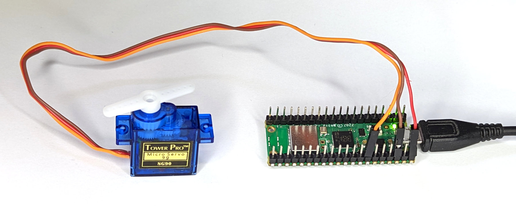
While the SG90 comes with it’s wires terminated in a 3 way du-pont connector, in order to make the connection to our header pins simple, replace the 3 way connector with three single pins.

Code

The code below will designate the GP pin to be used as an output (GP28) and the frequency of the signal (50Hz (which equates to a period of 20ms)).

The aim is to sweep the servo through an arc of 180 degrees and then back again.

We then use two while loops to move the servo from a pulse width of 0.52ms to 2.6ms and then back again in an endless loop. Now, I’ll be the first to admit that this does not equate with the expected values of 1ms and 2ms. I have selected the values in the code, because that’s what roughly equates to the -90 and +90 degrees of movement. Why is it not nore accurate? Good question. I tried a few iterations including using duty_u16 (from 3277 to 6554) instead of duty_ns, but it still didn’t seem to work accurately. I suppose my takeaway is that the servo is particularly cheap and maybe I got what I paid for. Irrespective, it was possible to manually calibrate the servo to discover appropriate values.

import time
from machine import Pin, PWM

pwm = PWM(Pin(28))
pwm.freq(50)

while True:
    for pulse in range(520,2600,10):
        pwm.duty_ns(pulse*1000)
        time.sleep_ms(5)
    for pulse in range(2600,520,-10):
        pwm.duty_ns(pulse*1000)
        time.sleep_ms(5)

Warning

I initially operated the servo in it’s sweeping motion while my cat was nearby. She quickly took an interest and had a bit of a play with it.

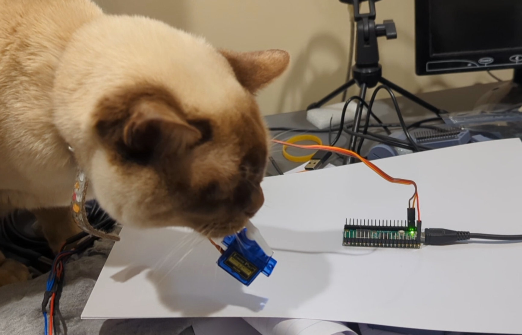
Later I heard a strange noise from the office and found her up on the desk investigating it some more. I have since found that I can operate it and she will quickly come and investigate what’s happening. In short, she’s obsessed. I now have to keep the office door shut.

So fair warning.

Controlling a Motor with the Raspberry Pi Pico

Being able to control a motor takes the principles of cross-over from a computing world to the physical world into a different dimension. Almost literally, because it provides the mechanism to induce movement and effect into the environment. Little wonder then at the excitement of building a robot or driving a tracked vehicle since it represents a direct engagement into the way that we (as humans) also interact with the world.

What are the principles of motor control?

A DC motor converts electrical energy into mechanical energy (and heat). It works on the principle that when a current carrying conductor is placed in a magnetic field, it experiences a mechanical force. It does this because the conductor generates a magnetic field of its own and the interaction of the two magnetic fields creates the force (this can be quantified by Flemings left hand rule). There are many different mechanisms and classifications associated with motor design, but those basic principles of current flow and interacting magnetic fields are the way that the motion is produced.

The two most common methods of controlling a DC motor are via varying an applied voltage level or by pulsing the voltage for varying lengths of time (Pulse Width Modulation (PWM)). PWM control is the most popular method because of the increased efficiency and easy of control over the motor. In effect PWM varies the motor speed by simulating a variation in supply voltage. These periodic pulses, when combined with a smoothing effect, makes the motor act as if it is being powered by an adjustable voltage.

The other common piece of the motor control puzzle is the use of what is called an ‘H Bridge’. This is a circuit comprised of four switches controlled in pairs. When either of these pairs are closed, they complete the circuit and subsequently power the motor with current running a different direction. This allows for direction control of the motor.

Don’t be misled by the overly simple explanation above of the motor control. It is a complicated topic that could be the subject of a lifetimes review and research, but feel happy with the concept of a varying electric current creating a magnetic field that in turn (see what I did there) interacts with another magnetic field to produce rotation.

It’s also worth mentioning that most of the above will be completely obscured from us as we can simply apply an appropriate signal to produce the required effect. Nonetheless, it’s useful to understand the very basics of what is happening and why.

How will we implement it?

Motor

Any list of requirements should start with the thing that will drive subsequent selection criteria. In this case we should start with the motor. We will use what are commonly called ‘TT Motors’. These are a simple combination of motor and gearbox in a plastic housing. They may or may not come with wires attached, and possibly a wheel(!) so select as appropriate. We will start with a specification for using two, since ultimately it would be good to use our project to build a device with the ability to drive two independent motors for direction control of a vehicle or similar.

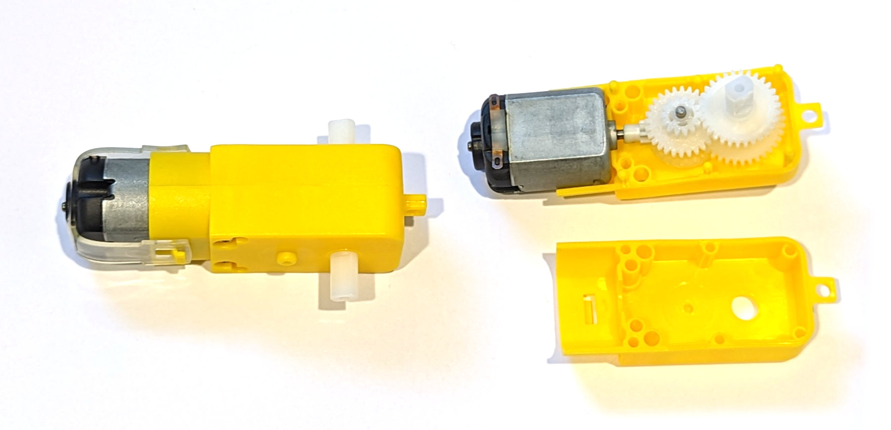
These motors can be operated with anywhere from 3v to 12V although the recommended range is from 3V to 9V. With 6V applied they will rotate at approximately 200rpm drawing 200mA. This is all assuming a ‘no-load’ condition where the motor is just turning it’s own shaft and not being put under strain (like driving a vehicle). When put under a load that resists the turning force of the motor it will draw up to 1.5A (at 6V) when forced to to a stall (stop).

Power

Running a motor takes a reasonable amount of current. Our Raspberry Pi Pico is not designed to pass significant amounts of current through it. The possible sources of electrical power from a Pico would be via either the VBUS (40) or 3V3 (36) pins.

• VBUS represent the micro-USB input voltage, connected to micro-USB port pin 1. This is nominally 5V, and the amount of current will be limited to the connected supply. While this might technically be a possible source, for power for a motor, it would only be suitable in situations where you were super careful about the type of motor and the USB power supply used. I wouldn’t do it and I don’t recommend it.
• The other option is from the 3V3 pin which is also the main 3.3V supply to RP2040. This pin can be used to power external circuitry, but the maximum output current that it can supply should be kept under 300mA. This is not realistically enough to power even a tiny DC motor.

In short, we won’t be taking the power supply for our motor from our Raspberry Pi Pico.

The sensible source for our power will be from an external battery or dedicated DC power supply. For the sake of simplicity we will use a simple 4 AA cell battery pack. This will be able to supply a voltage close to our 6V nominal identified for the motors. It should be able to supply over 1A, although running it under that much load for an extended period will reduce the voltage quickly)

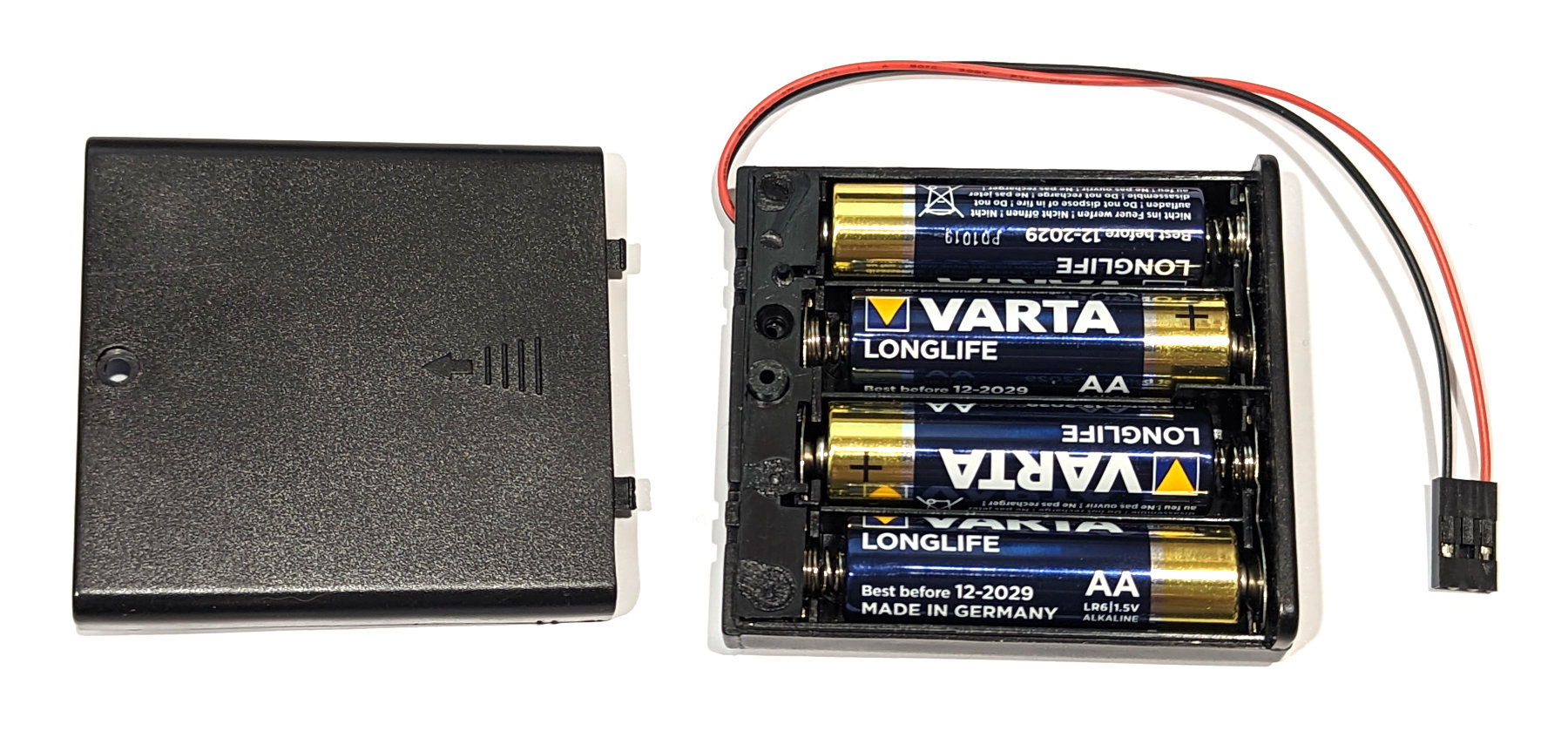
If we were making this a stand-alone project (for a robot or vehicle), we would probably use this as the source for the power for the Pico as well (with a suitable regulator). Likewise, if this was for a project that was intending to be used a lot, we should consider some form of rechargeable option.

Controller / Driver

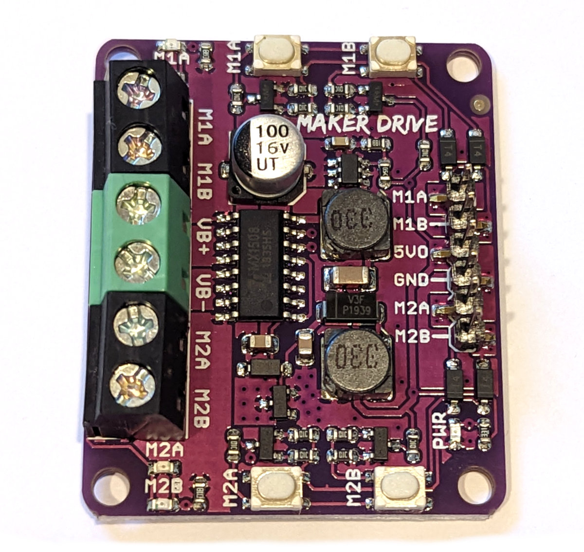
So from our requirements gathering process above we want to have a motor driver / controller that can supply two motors with a peak output of 1.5A per motor (just in case), it should be able to accept 6V input and in an ideal world it would act as a supply for our Pico with 5V out.

With these requirements in mind I have selected the Maker-Drive board from Cytron. It meets our requirements nicely and is very reasonably priced.

Types of Motion

There are two objectives that we will want to achieve with our motor control. The first will be simple movement forwards, backwards and stopped. The second will be to adjust the speed of any movement.

Simple movement

The simplest form of control is making our motor turn clockwise, anticlockwise or to have it stop.

Nost DC motor controllers will use two control signals to accomplish this. Either control signal can be high or low and therefore, any combination of the two will provide us with with four different signal combinations.

As we can see form the table above, whenever any of the two signals are both high or both low the motor will be stopped and whenever the signals are different it will be rotating.

Variable Speed

To vary the speed of our motor we need to apply Pulse Width Modulation (PWM) to our control signals. When the motor is turning in the simple example above, one of the control signals is set low and the other high. To vary the speed we can ‘pulse’ (modulate) the high pin off and on very quickly so that when combined with a smoothing effect, the voltage will appear reduced to the motor. The way that we will control this voltage is by varying the ‘duty cycle’ of the pulses.

The duty cycle of a signal is commonly expressed at the ratio of the time that the signal is high compared to the total period of one cycle. Thus a 70% duty cycle means the signal is on 70% of the time but off 30% of the time.

In MicroPython (as we will see in the code that follows) the duty cycle can be set as a parameter called duty_u16 where it varies between 0 (0% duty cycle) to 65535 (100% duty cycle).

Connecting Up the motor controller and battery

Connecting up our various components is as much about following a logical approach as it is about keeping everything simple.

The battery pack has its positive and negative connections connected to the VB+ and VB- pins of the Maker Drive board

The motor is connected to the M1A and M1B screw in connections on the Maker Drive. This will send the voltage out to the motor. It doesn’t matter which way round you connect the wires to the motor as it will be difficult to determine which direction the motor will turn before you test it. The rule of thumb here is that we will connect up our motor and test it and then change the connection if it is turning in the wrong direction.

The Pico has two PWM connection enabled pins connected (every GPIO pin can be configured as a PWM output) to the Maker Drive M1A and M1B header pins. In the case of the diagram below we are using GPIO pins 4 and 5 (physical pins 6 and 7). We also need to connect up a ground connector between the Maker Drive and the Pico.

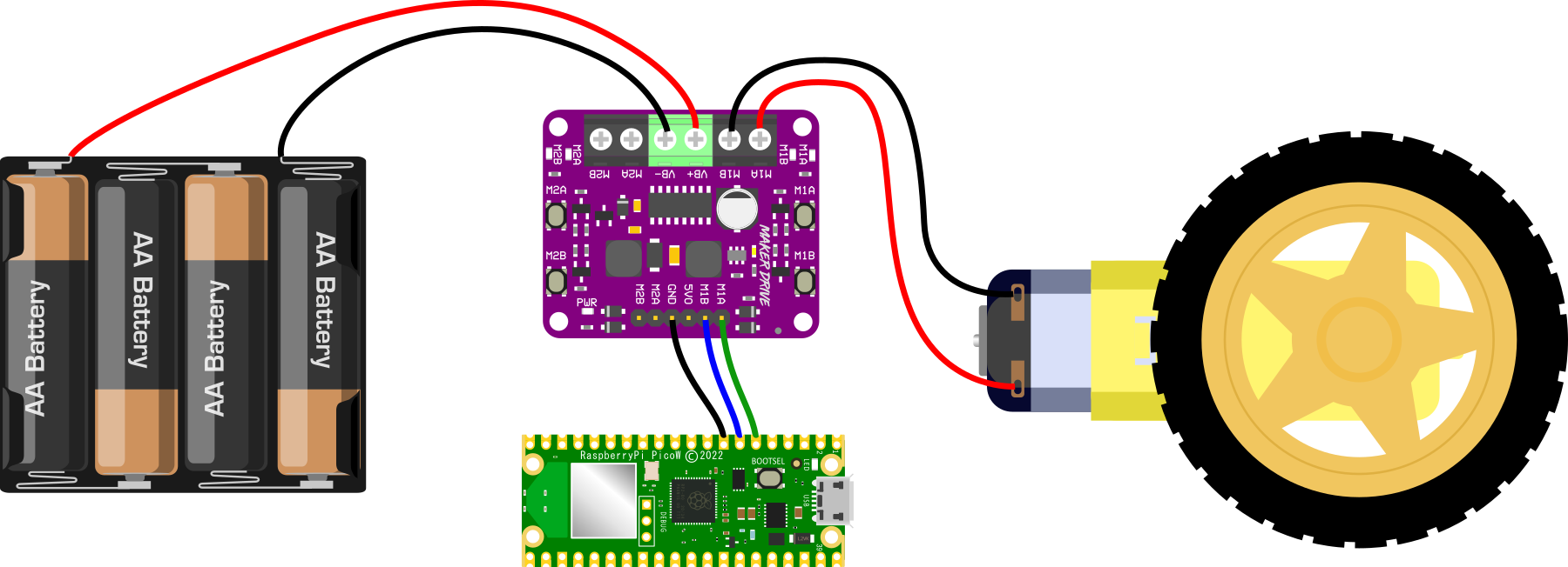
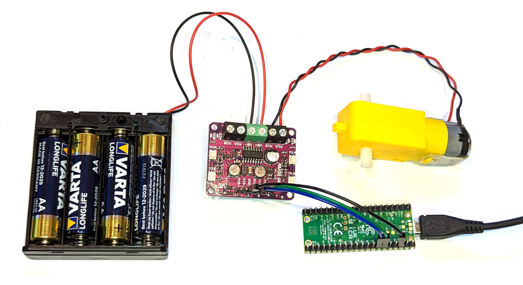
The connection above is assuming that we still have our Pico connected via USB to our computer for programming and testing. If we get to a point where we want to operate the Pico and the entire ensemble independently, we can also connect the Maker Drive 5VO pin to the VBUS pin (40) on the Pico and the Pico will take it’s power from the Maker Drive board which is in turn taking its power from the battery pack.

While the higher current connections to the Maker Drive board will go to the screw terminals, the connections that carry lower power (like the signalling) can be connected using Dupont connectors. A practical example of that can be seen below.

Code

The two different approaches to controlling the motors are outlined below.

Simple constant speed approach

The code below is a simple test which runs the motor forward and then backward for two second each way.

import time
from machine import Pin

motor1a = Pin(4, Pin.OUT)
motor1b = Pin(5, Pin.OUT)

# Forward
motor1a.high()
motor1b.low()

time.sleep(2)

# Backward
motor1a.low()
motor1b.high()

time.sleep(2)

# Stop
motor1a.low()
motor1b.low()

Variable speed demonstration

The code below is demonstrates the ability to vary the speed of the motor by using pulse width modulation on the signals.

import time
from machine import Pin, PWM

motor1a = Pin(4, Pin.OUT)

pwm_motor1b = PWM(Pin(5))
pwm_motor1b.freq(50)

# 1/4 speed
motor1a.low()
pwm_motor1b.duty_u16(16383)
time.sleep(2)

# 1/2 Speed
motor1a.low()
pwm_motor1b.duty_u16(32767)
time.sleep(2)

# FULL SPEED!!!!
motor1a.low()
pwm_motor1b.duty_u16(65535)
time.sleep(2)

# Stop
motor1a.low()
pwm_motor1b.duty_u16(0)

Using a Stepper Motor with a Raspberry Pi Pico

The Stepper Motor

A stepper motor is a type of electric motor that rotates in precise increments or ‘steps’ when electrical commands are applied. Stepper motors are commonly used in applications where precise positioning is required, such as in printers, scanners, and 3D printers.

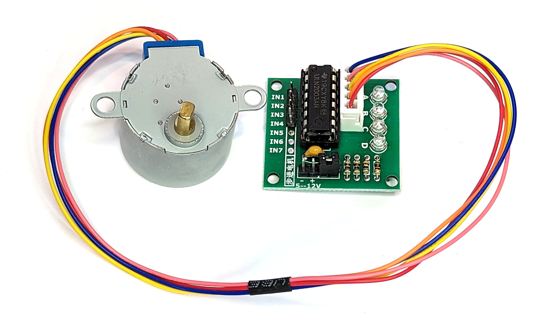
Stepper motors can be classified as either unipolar or bipolar. Unipolar stepper motors have a single winding per phase and require a special type of drive circuit, while bipolar stepper motors have two windings per phase and can be driven with a more common H-bridge drive circuit.

Stepper motors operate by energizing the windings in a specific sequence, causing the rotor to rotate a precise number of degrees per step. The number of steps per revolution and the step angle (the angle of rotation per step) are typically specified by the manufacturer. Stepper motors can be controlled with a microcontroller or other type of controller, such as a motor driver or stepper motor driver.

There are several key differences between a stepper motor and a normal (also known as a brushed or brushless DC) motor:

• Precise positioning: Stepper motors are capable of more accurate positioning because they rotate in precise increments or “steps” when electrical commands are applied. Normal motors, on the other hand, are not capable of precise positioning because they rotate continuously when powered.
• Torque: Stepper motors typically have less continuous torque than normal motors, but they can deliver high torque in short bursts. Normal motors, on the other hand, can deliver a more consistent level of torque over a longer period of time.
• Speed: Stepper motors have a limited speed range, typically up to several hundred RPM, depending on the model. Normal motors, on the other hand, can reach higher speeds and have a wider speed range.
• Control: Stepper motors can be controlled with a microcontroller or other type of controller, such as a motor driver or stepper motor driver. Normal motors typically require a more complex drive circuit, such as an H-bridge, to control the speed and direction of rotation.
• Cost: Stepper motors tend to be more expensive than normal motors of similar size and power due to their precision and control capabilities.

Putting the ‘Step’ into stepper motors

Stepper motors operate by energizing their windings in a specific sequence, causing the rotor to rotate a precise number of degrees per step. The number of steps per revolution and the step angle (the angle of rotation per step) are typically specified by the manufacturer.

• The controller sends electrical commands to energize the windings in a specific sequence. For example, the sequence may be to energize winding A, then winding B, then winding C, and finally winding D.
• When the windings are energized, the magnetic fields generated by the windings interact with the magnetic field of the permanent magnets in the rotor, causing the rotor to rotate a certain number of degrees.
• The controller sends the next set of electrical commands to energize the windings in the next sequence. For example, the sequence may be to energize winding C, then winding D, then winding A, and finally winding B.
• The process repeats, with the controller sending electrical commands to energize the windings in the specified sequence, causing the rotor to rotate a certain number of degrees each time. This results in the stepper motor turning in a precise, step-by-step manner.

The specific sequence of the windings being energized depends on the type of stepper motor (unipolar or bipolar) and the specific drive circuit being used.

Torque

Rated torque is a measure of the maximum torque that a stepper motor can produce under specified conditions. It is typically expressed in units of force times distance, such as Newton-meters (Nm) or ounce-inches (oz-in).

Rated torque determines the amount of force that the motor can generate to move a load. In general, a stepper motor with a higher rated torque will be able to move a larger or heavier load than a motor with a lower rated torque.

It is important to note that the rated torque of a stepper motor is not constant and can vary depending on factors such as operating voltage, current, speed, and temperature. In general, the rated torque of a stepper motor decreases as the speed increases, and it may also be affected by the type and size of the load being driven.

The 28BYJ-48

The 28BYJ-48 is a small, low-cost stepper motor commonly used in hobbyist and educational projects. It has a 5V operating voltage and is driven by a ULN2003A driver board (or similar stepper motor driver).

The 28BYJ-48 has a step angle of 5.625 degrees and a step resolution of 64 steps per revolution, resulting in a total of 4096 steps per revolution. It has a rated torque of 44.4 g-cm (0.6 oz-in) and a maximum no-load speed of approximately 15 RPM.

The 28BYJ-48 is a unipolar stepper motor, meaning it has a single winding per phase and requires a special type of drive circuit to operate (hence the use of the ULN2003A driver board). It is commonly used in applications such as small robotics, educational models, and DIY projects.

Connecting the Pico to the controller to the GY-521

The connection from the ULN2003A driver board to the motor is via a pre-made molex connector. Power is applied to the ULN2003A via the + and - connectors which should be connected to a 5V supply. In the connection diagram below that power is being sourced from the VBUS connector of the Raspberry Pi Pico. We need to be a little bit careful here. The 28BYJ-48 is quite power hungry (around 240mA) and typically this should come from a separate power source. However, in this case, the VBUS connector on the Pico is connected directly to the 5V supply from the USB connector and so long as that has sufficient power we should be alright. Having said that, be aware that this is a very simple motor and it will consume power even when it is standing still. If we leave it for a few minutes, we can feel it getting warm.

The power connections are as follows;

• VBUS (Pin 40) -> +
• GND (Pin 38) -> -

The 28BYJ-48 rotates by sending signals to its four coils in a specific sequence that switches the coils on and off in a pattern that creates a magnetic field that rotates the motor. Those four coils are controlled from four GPIO pins on the Pico. In our case we will use GPIO18, 19,20 and 21. For no reason other than they make drawing the circuit diagram below slightly prettier.

The connections are as follows;

• GPIO18 (Pin 24) -> IN1
• GPIO19 (Pin 25) -> IN2
• GPIO20 (Pin 26) -> IN3
• GPIO21 (Pin 27) -> IN4

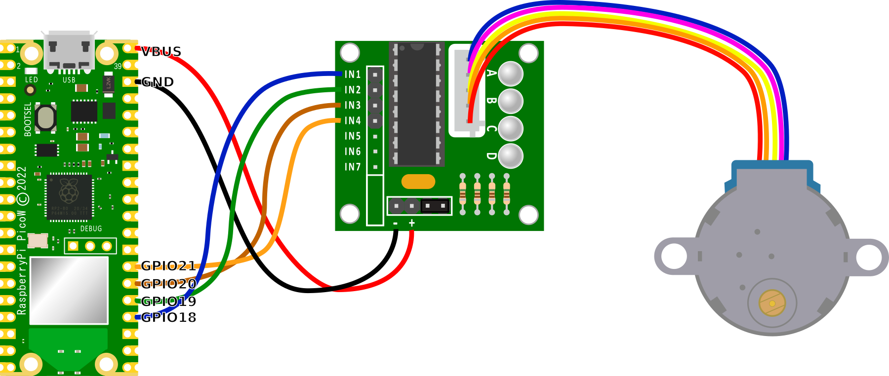
Code

The following code demonstrates the stepper motor turning in one direction;

from machine import Pin
from time import sleep

IN1 = Pin(18,Pin.OUT)
IN2 = Pin(19,Pin.OUT)
IN3 = Pin(20,Pin.OUT)
IN4 = Pin(21,Pin.OUT)

pins = [IN1, IN2, IN3, IN4]

sequence = [[1,0,0,0],[0,1,0,0],[0,0,1,0],[0,0,0,1]]

while True:
    for step in sequence:
        for i in range(len(pins)):
            pins[i].value(step[i])
            sleep(0.001)

The following code allows the motor to turn in different directions through a function call;

import time
from machine import Pin

# Constants for the stepper motor pins
IN1 = Pin(18, Pin.OUT)
IN2 = Pin(19, Pin.OUT)
IN3 = Pin(20, Pin.OUT)
IN4 = Pin(21, Pin.OUT)

# Sequence for moving the stepper motor
SEQUENCE = [[1,0,0,0], [0,1,0,0], [0,0,1,0], [0,0,0,1]]

# Function to move the stepper motor
def move_stepper(direction, steps):
    # Set the input pins
    pins = [IN1, IN2, IN3, IN4]

    # Set the direction of the sequence
    if direction == 'forward':
        sequence = SEQUENCE
    elif direction == 'backward':
        sequence = list(reversed(SEQUENCE))

    # Loop through the specified number of steps
    for i in range(steps):

        # Set the input pins based on the current step
        for j in range(len(pins)):
            pins[j].value(sequence[i%4][j])

        # Delay between steps
        time.sleep(0.005)

# Main loop
while True:
    # Move the stepper motor forward
    move_stepper('forward', 400)

    # Move the stepper motor backward
    move_stepper('backward', 400)

Connecting an SD Card to the Raspberry Pi Pico

The Raspberry Pi Pico is a very capable device, but it lacks the ability to store sizeable amounts of data on the board. This is a useful function when using the Pico for tasks such as data logging. To make this function practical we can use an SD card for expanding storage via an adapter.

SD cards are great for storing logging and data from microcontroller projects that can then be read on a computer.

We can use SD cards in Serial Peripheral (SPI) mode which allows us to rely on easy to use SPI peripherals and libraries for communication. SPI mode is perfect if we’re writing short amounts of data to a file (e.g. event logging).

SD card adapter or adaptor.

First the elephant in the room. Whether you spell it adapter or adaptor, it means the same thing. Let’s not get hung up on the semantics of language usage. As a gesture of improving international relations (or perhaps it’s just a personal weakness) I will spell it both ways, although I tend to lean towards adapter.

My personal SD Card adapter journey

I’ll be the first to admit that I haven’t exactly got a large amount of experience in using SD card adapters, but while going the through the process of testing different adapters and cards, I came across a few inconsistencies. This varied between adapters and card types. With that in mind, stay flexible and be patient. Have a range of cards on hand, and don’t be afraid to try something new like rolling your own adapter made out of a standard adapter and some header pins. Also try to start from a consistent baseline with a freshly formatted SD card, ensuring that it’s formatted using the FAT32 file system. And while we’re here, we can’t do anything fancy like having multiple partitions on our SD card. There can be only one! (Gratuitous Highlander reference)

Choose your weapon

While writing this section I used a few different adapters. From the range below I had consistently good results from the smaller adapter and the ghetto version that I created from a traditional adapter and some header pins. I never got results that I was happy with using the larger circuit board version. This might have been some combination of software, hardware and my own personal incompetence, but there it is.

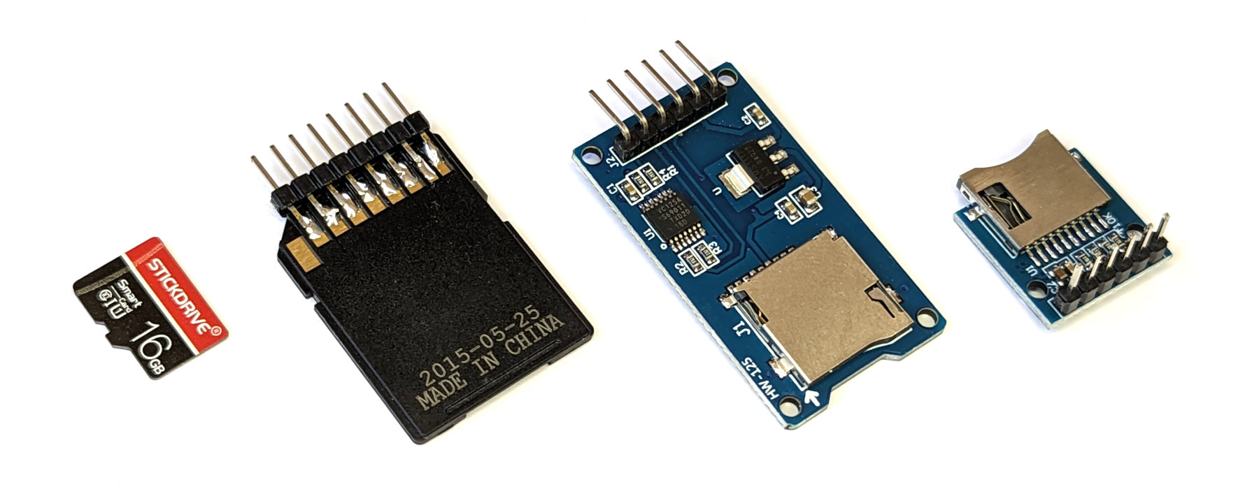
Install the SDCard Library.

The modules for supporting SD card use are not yet (as at 2022-10-31) built into the MicroPython distribution for the Pico, so we can add them simply enough manually (once they are included, if an observant reader notices before I do, could you let me know and I will update this section of the book :-))

To make use of the module we will need to download it from GitHub and then copy it over to our Pico. I found this most easily accomplished by first downloading the file to the main computer and then going File >> Open on Thonny and selecting the appropriate file. From there go File >> Save as… and select the Pico as the location to save the file (making sure to save it with the appropriate name (sdcard.py))

Connect the SD Card Adapter

The Serial Peripheral Interface (SPI) utilises four physical connections. Typically on an adapter they will be labelled as such;

• SCK: Serial Clock
• MOSI: Master Out Slave In
• MISO: Master In Slave Out
• CS: Chip Select

In turn they will be connected to one of the sets of SPI connections on the Raspberry Pi Pico. In our case we will use controller 0 (the pico has two controllers and four sets of possible connections to the GPIO pins) and GPIO pins 16 - 19

• SPI0 RX (GPIO16) <-> MISO: Master In Slave Out
• SPI0 CSN (GPIO17) <-> CS: Chip Select
• SPI0 SCK (GPIO18) <-> SCK: Serial Clock
• SPI0 TX (GPIO19) <-> MOSI: Master Out Slave In

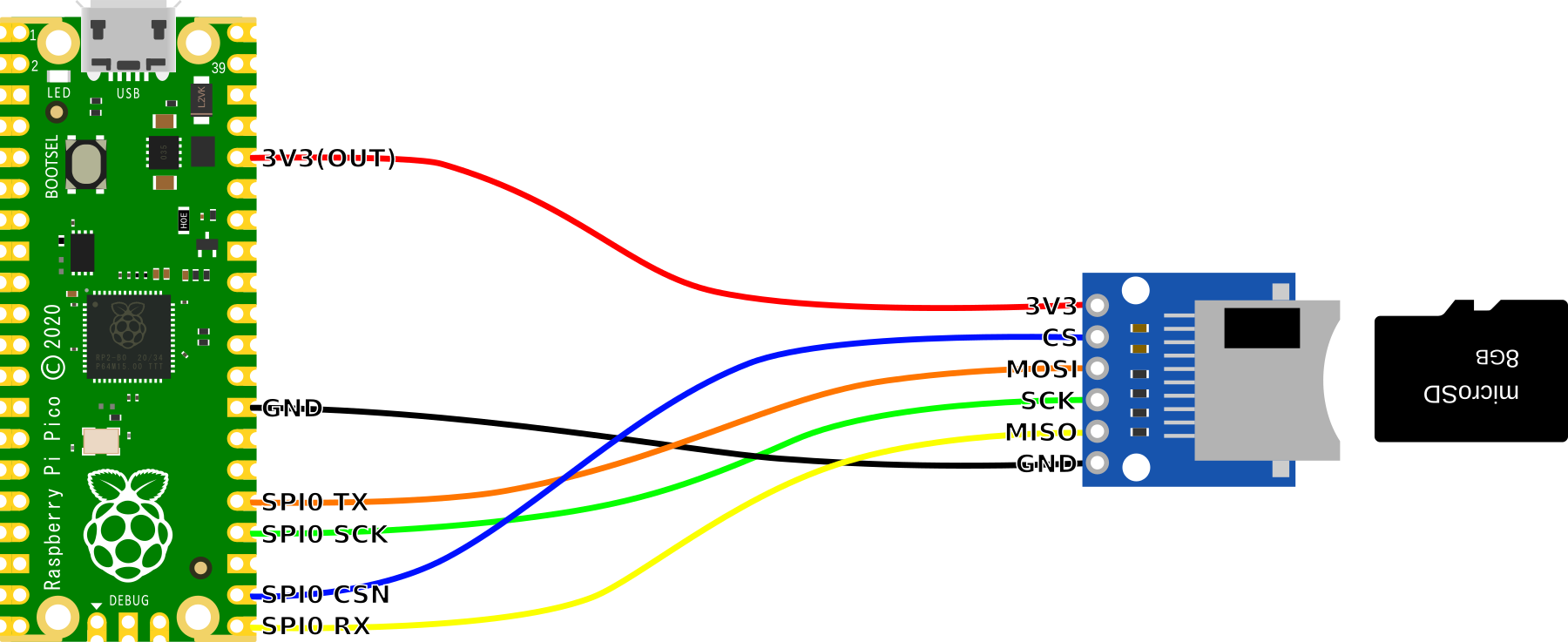
Of course we also connect up or 3.3V and ground connections.

In a practical sense, connecting up with Dupont connectors is a simple method to test functionality.

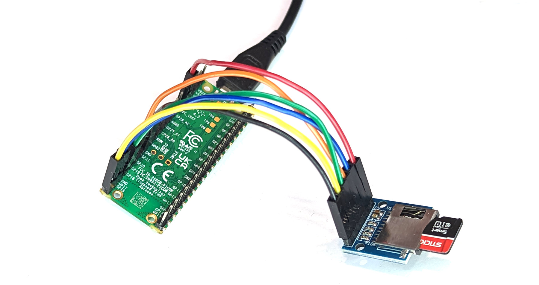
Code

In a new new document, enter the following code:

import machine
import sdcard
import os

# Set the Chip Select (CS) pin high
cs = machine.Pin(17, machine.Pin.OUT)

# Intialize the SD Card
spi = machine.SPI(0,
                  baudrate=1000000,
                  polarity=0,
                  phase=0,
                  bits=8,
                  firstbit=machine.SPI.MSB,
                  sck=machine.Pin(18),
                  mosi=machine.Pin(19),
                  miso=machine.Pin(16))
sd = sdcard.SDCard(spi, cs)

# Mount filesystem
vfs = os.VfsFat(sd)
os.mount(vfs, "/sd")

# Create a file in write mode and write something
with open("/sd/sdtest.txt", "w") as file:
    file.write("Hello World!\r\n")
    file.write("This is a test\r\n")

# Open the file in read mode and read from it
with open("/sd/sdtest.txt", "r") as file:
    data = file.read()
    print(data)

Make sure you have the SD card inserted into the breakout board and click the Run button. You should see the contents of the file that is created (sdtest.txt) printed out in the shell. We can go one step further and eject the SD card from the adapter and plug it into our desktop machine where we can browse to the file and read it from the computer.

Our code above has the feature of creating the file sdtest.txt when it writes to it. This also means that it will overwrite the file every time it is run. If we want to append information to an already existing file we can use an a instead of a w. Something similar to the below would do the trick placed between the write and read blocks;

# Append information to a file
with open("/sd/sdtest.txt", "a") as file:
    file.write("With even more information!\r\n")

If we were utilising the SD card as a store for a data logging application, we would be appending information.

Bonus Connection!

If you’re keen to DIY you can solder header pins to a more traditional SD to Micro SD card adapter and connect that up to our Pico. I was a little sceptical before trying it out, but it worked like a charm.

With that in mind, here is a connection diagram for when you have mastered your soldering skills.

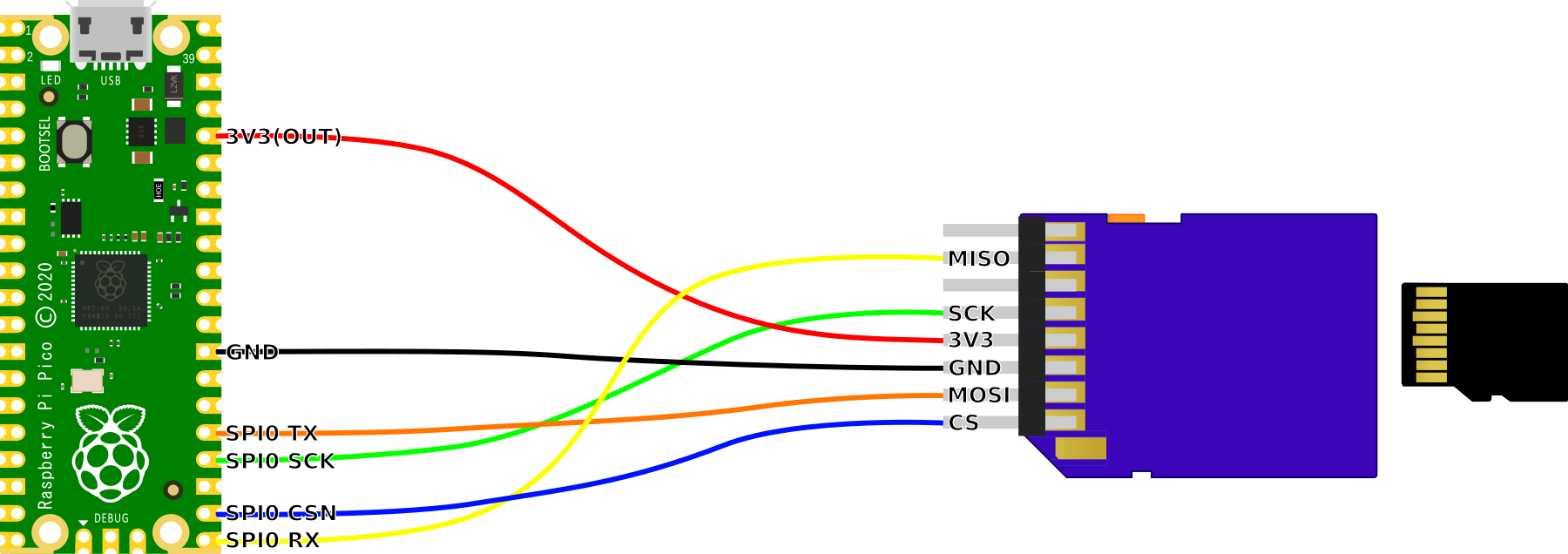
Connecting MQ Series Gas Detectors to the Pico

This project will measure the presence of types of gas in the air using one of the MQ series of sensors.

The Sensor

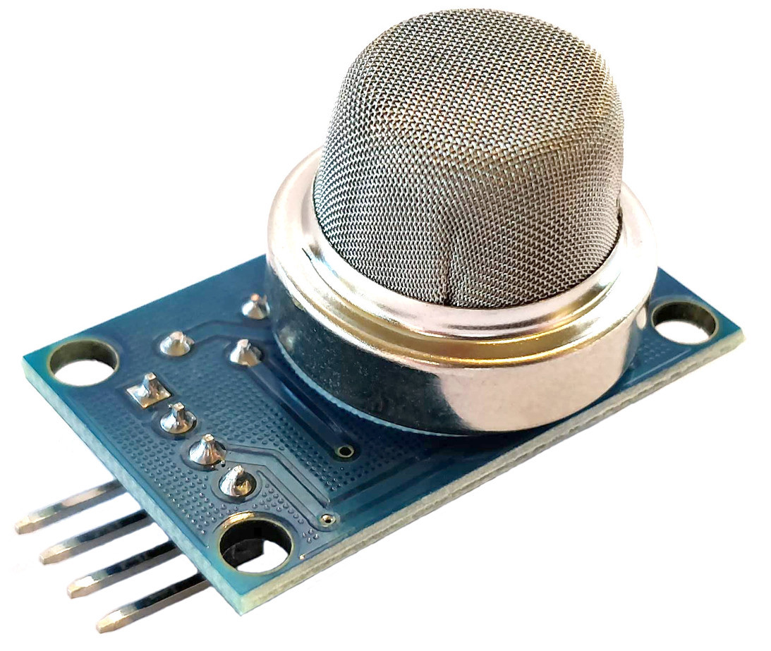
The MQ-2 is a commonly used gas sensor in MQ sensor series. It is what’s referred to as a Chemiresistor as the detection is based upon change of resistance of the sensing material when the gas comes in contact with a Metal Oxide Semiconductor (MOS). The value of the analog signal output varies as the gas concentration varies.

Different metal oxides have different chemiresistive properties allowing them to sense different gasses.

The most obvious feature of the sensor is the surrounding layer (actually two layers) of stainless steel mesh called an ‘anti-explosion network’. This is present to make sure that the heater element inside the sensor doesn’t cause an explosion while it is in the presence of flammable gasses. It also acts as a filter to allow only gases to pass through to the sensor.

The MQ-2 sensor which we will be using can detect LPG, butane, propane, methane, alcohol, Hydrogen and smoke concentrations from 200 to 10000ppm.

There are a wide range of sensors in the MQ series that can detect the presence of different gasses.

The sensor we will be using is mounted on a circuit board for ease of connection. We provide it with a 3.3VDC supply and it returns an analog signal that varies in proportion to the concentration of our target gas. That signal can vary between 0VDC and 3.3VDC. The board also includes a digital output option, but this is designed to provide a breakpoint level of gas, rather than a value. The variable resistor (potentiometer) on the board allows this breakpoint to be varied.

The connections on the board are as follows

• VCC: Is the power input. This will require 3.3VDC in our case, but it can actually accept anywhere from 2.5VDC to 5VDC)
• GND: Is the ground pin
• DO: Provides the digital output set by the potentiometer
• AO: is the analog output signal.

It is this analog voltage that is then digitised with our Analog to Digital Converter (ADC) that is built into the microcontroller.

Connect Everything Up

We will want to connect;

• VCC on the MQ-2 to the 3V3 pin (36) on the Pico
• GND on the MQ-2 to the Ground pin (38) on the Pico
• A0 on the MQ-2 to ADC0 pin (31) on the Pico

The power and ground pins are fairly self explanatory, and because the MQ-2 has an analog output that will vary from the applied voltage to 0V, we will apply this to one of our Analog to Digital Converter (ADC) pins. In this case ADC0 on pin 31.

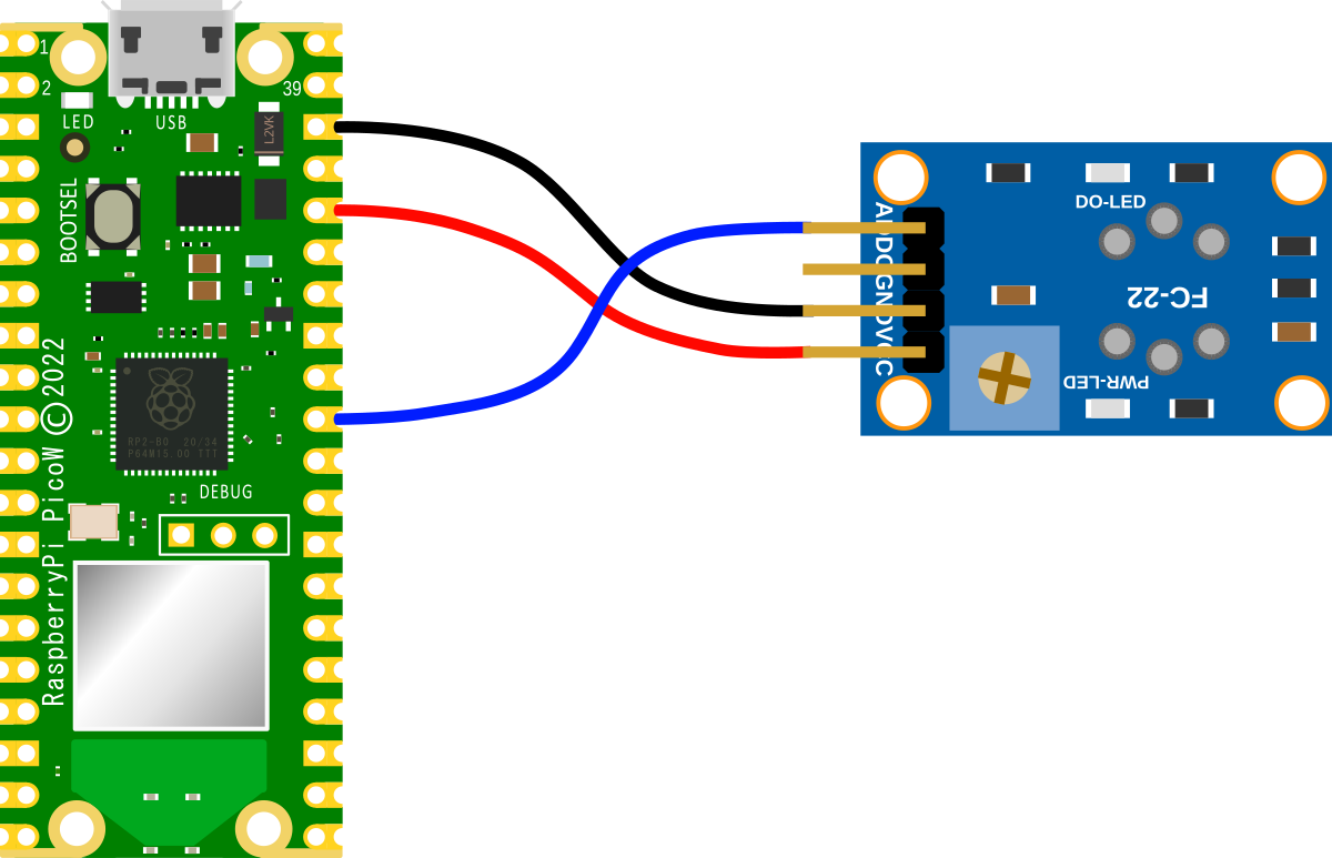
Connecting the sensor practically can be achieved in a number of ways. But because the connection is relatively simple we can build a minimal configuration that will plug directly onto the pins using Dupont header connectors and jumper wire.

Code

The following code will read the value from the MQ-2 and convert that to the effective voltage that should be present on the analog pin. It will print this out every second.

import machine
import time

mq2 = machine.ADC(26)
conversion_factor = 3.3 / (65535)

while True:
    voltage = mq2.read_u16() * conversion_factor
    print("Output voltage is",voltage)
    time.sleep(1)

Distance Measurement using Time of Flight Sensor

What is a Time Of Flight Sensor?

A Time of Flight (ToF) sensor measures the time it takes for a signal to travel a distance through a medium. This is a deliberately broad definition since there are different ways to carry this out depending on the application. For the purposes of our explanation we are going to be describing a sensor that measures the time elapsed between the emission of a pulse of light, its reflection off an object, and its return to the ToF sensor.

In this case, the sensor itself is an extremely compact device that is popular for applications in robotics and cameras.

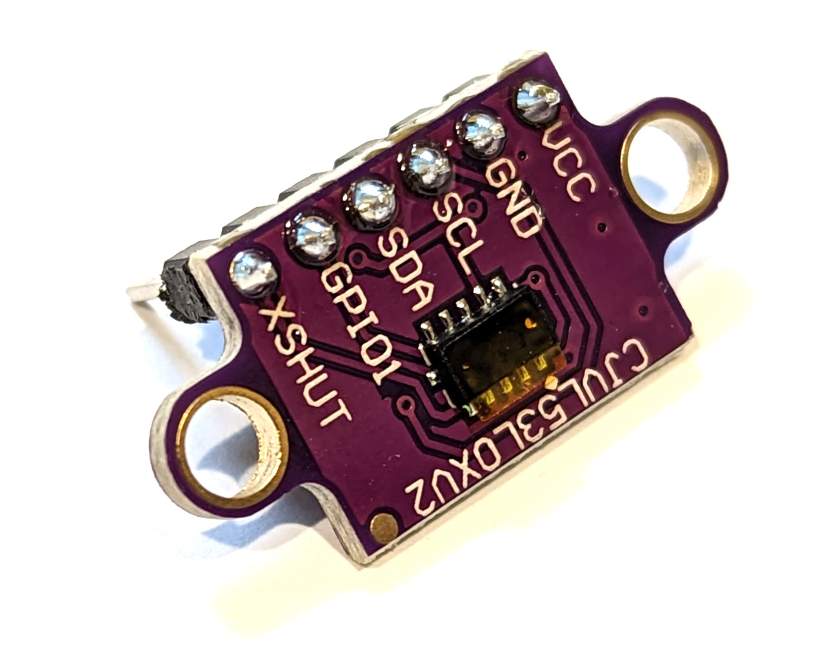
The sensor we will be using is a VL53L0X Time-of-Flight laser-ranging module which can provide an accurate distance measurement to objects up to 2m away.

The VL53L0X uses a 940nm (infrared) Vertical Cavity Surface-Emitting Laser which is invisible to the human eye. The output is engineered to remain within Class 1 laser safety limits and as such is safe under all operating conditions. Have a read of the vl53l0x Datasheet for all the good info.

How does a Time Of Flight Sensor Work?

ToF sensors use a laser to emit infrared light. The light reflects off any object it strikes and returns to the sensor. Based on the time difference between the emission of the light and its return it is able to measure the distance between the object and the sensor.

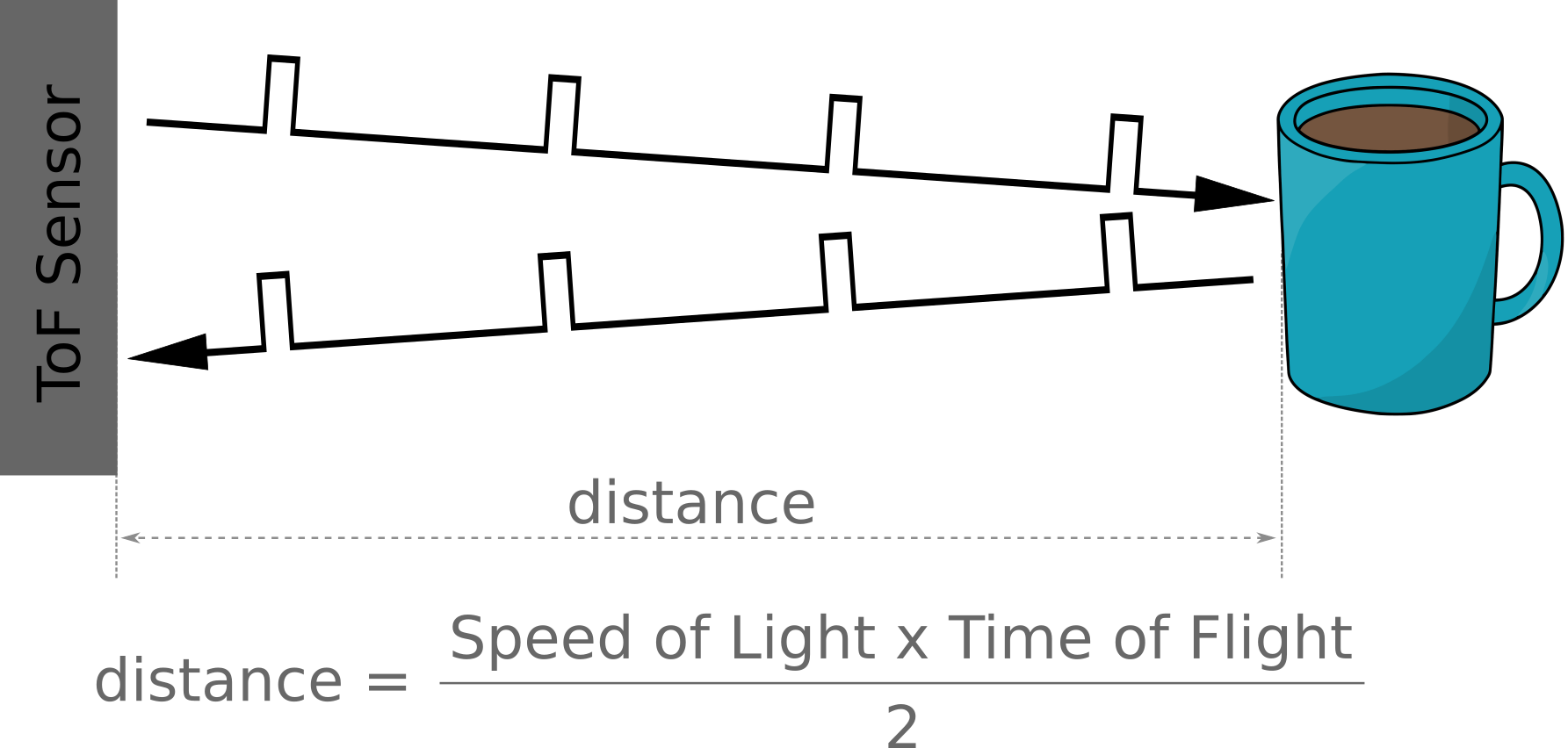
The VL53L0X precisely measures how long it takes for emitted pulses of infrared laser light to reach the nearest object and be reflected back to a detector, so it can be considered a tiny, self-contained lidar system. The sensor can measure distances of up to 2m with 1 mm resolution, but its effective range and accuracy depend on ambient conditions and target characteristics like size and degree of reflectivity. The sensor’s accuracy can vary from ±3% at best to over ±10% in less optimal conditions.

The beam of the emitted light is quite narrow and the orientation of the sensor and the measured object will be factors in recording accurate values. This is also a positive thing since the narrow light source is good for determining distance of only the surface directly in front of it. Unlike audio based systems that utilise ultrasonic waves, the ‘cone’ of sensing is very narrow.

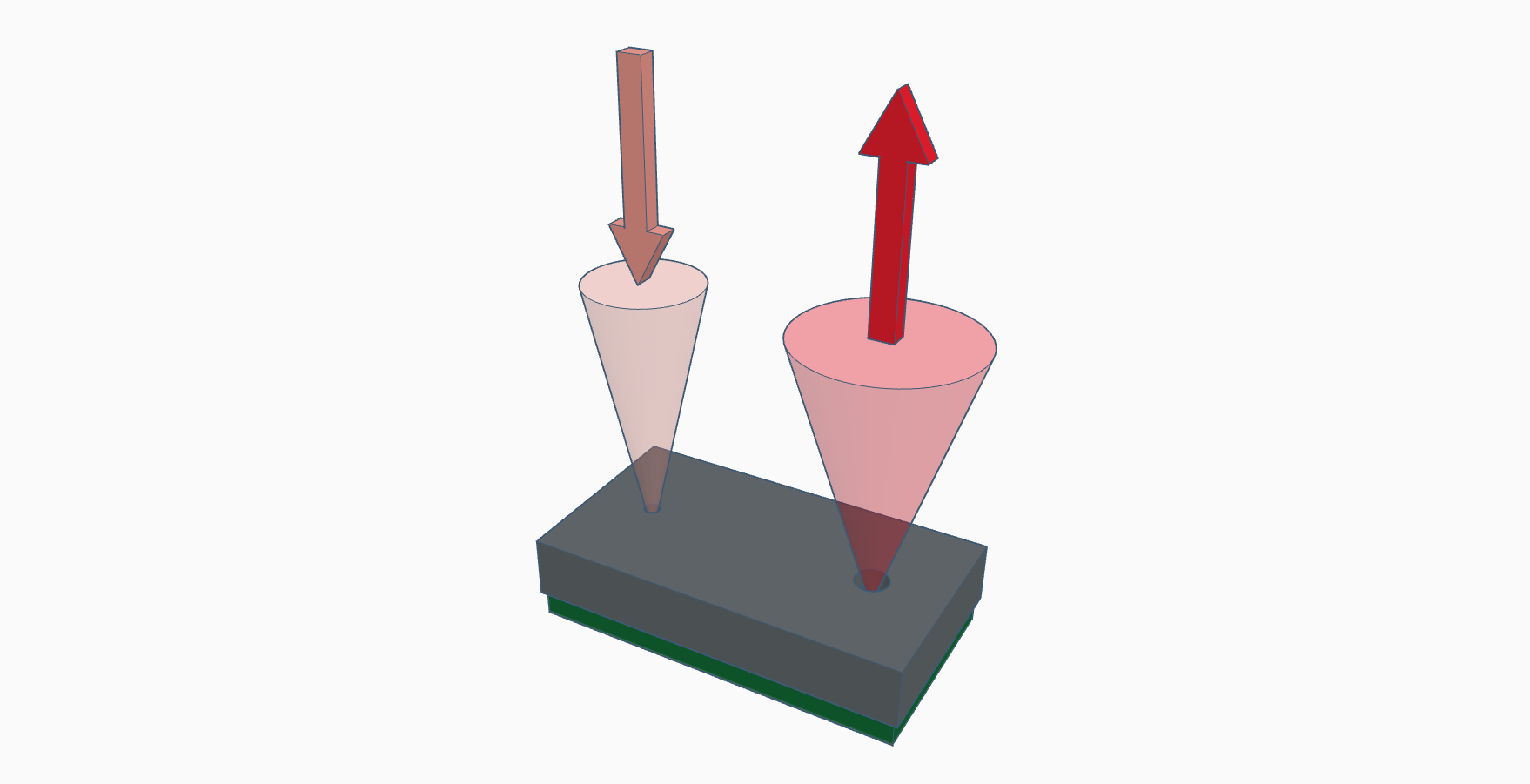
How is a Time Of Flight Sensor Controlled?

The sensor is controlled via I2C, but we can abstract the complexities of this via a prebuilt MicroPython module. This was initially developed by Robin Matzner and was then adapted by Kevin McAleer. To make use of the module we will need to download it from GitHub and then copy it over to our Pico. I found this most easily accomplished by first downloading the file to the main computer and then going File >> Open on Thonny and selecting the appropriate file. From there go File >> Save as… and select the Pico as the location to save the file (making sure to save it with the appropriate name (vl53l0x.py))

Because of the abstraction afforded by the library, the adjustments that we can make are nicely simplified.

Range Timing Budget

The first thing we can adjust is the range timing budget. This is set up to manage the ‘ranging phase’ of the measurement where, several pulses are emitted, then reflected back by the target object, and detected by the receiving array. The typical timing budget for a range timing budget is 33ms with 200ms being used for high accuracy and 20ms recommended for high speed. This is changed in the MicroPython code via the line;

tof.set_measurement_timing_budget(100000)

Pulse Period

The other major adjustment that we can introduce is to the period of the pulse that is send out. The shorter the pulse, the better for closer measurements, the longer the pulse, the better for more distant measurement. There are two period ‘types’, Pre Range (Type 0) and Final Range (Type 1). Longer periods increase the potential range of the sensor. Valid values are even numbers only. These can be set in the MicroPython code via the lines;

tof.set_Vcsel_pulse_period(tof.vcsel_period_type[0], 18)
tof.set_Vcsel_pulse_period(tof.vcsel_period_type[1], 14)

The Pre Range settings can go from: 12 to 18 (default is 14) and the Final Range settings can go from 8 to 14 (default is 10).

Connecting a Time Of Flight Sensor Up to the Pico

The connection is fairly simple with only four connections being required. Power, ground, Serial CLock line (SCL) and Serial DAta line (SDA). The following connections are used for this example;

• VL53L0X GND to Ground (pin 38) on the Pico (Black)
• VL53L0X VCC to the 3V3(OUT) (pin 36) on the Pico (Red)
• VL53L0X SCL to I2C1 SCL (pin 32) on the Pico (Orange)
• VL53L0X SDA to I2C1 SDA (pin 31) on the Pico (Brown)

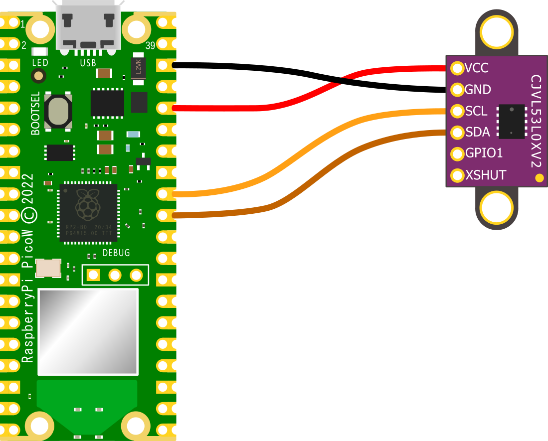
When selecting the I2C connections on the Pico, because the RP2040 microcontroller has two I2C controllers we need to ensure that we define which controller we are using in the code. I2C0 = id 0 and I2C1 = id 1. This is set in the following lines in the MicroPython code;

id = 1

i2c = I2C(id=id, sda=sda, scl=scl)

The best place to ensure that we have the id correctly identified is on the pinout.

Assuming that we have header pins soldered onto our Pico and the ToF sensor, the easiest ways to make a connection is via Dupont connectors.

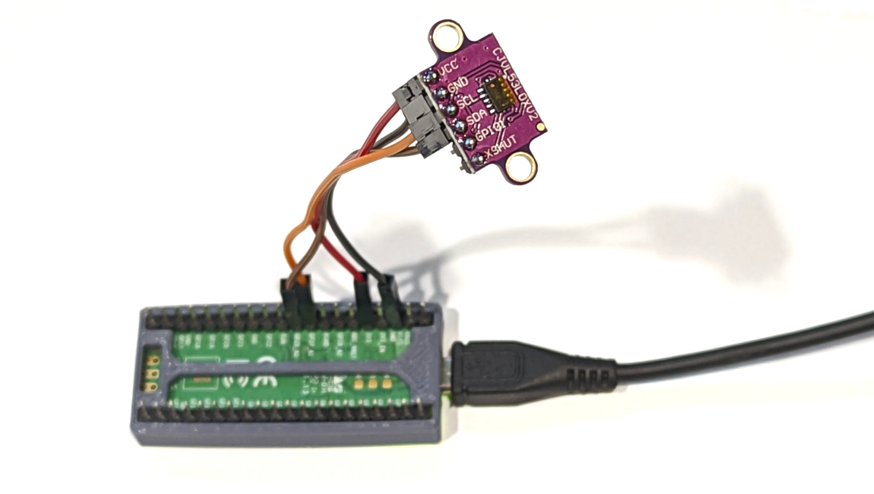
The only other point to note is that there are reports of some inconsistent measurements if the XSHUT pin is left ‘floating’ (i.e, not tied to a low (ground) or high pin). I haven’t experienced this myself, but if you’re seeing something that you can’t explain, this could be worth investigating

Code

The code below is largely that written by Kevin McAleer and published on GitHub. However, it is adapted to provide for the connection as described above and it is tuned to optimise for longer distance readings. Likewise I have included a small piece of code to average out the readings to improve consistency.

import time
from machine import Pin, I2C
from vl53l0x import VL53L0X

print("setting up i2c")
sda = Pin(26)
scl = Pin(27)
id = 1

i2c = I2C(id=id, sda=sda, scl=scl)

print(i2c.scan())

print("creating vl53lox object")
# Create a VL53L0X object
tof = VL53L0X(i2c)

# the measuting_timing_budget is a value in micro seconds, the
# longer the budget, the more accurate the reading. (originally 40000)
budget = tof.measurement_timing_budget_us
print("Budget was:", budget)
tof.set_measurement_timing_budget(100000)

# Sets the VCSEL (vertical cavity surface emitting laser) pulse period
# for the given period type (VL53L0X::VcselPeriodPreRange or
# VL53L0X::VcselPeriodFinalRange) to the given value (in PCLKs).
# Longer periods increase the potential range of the sensor. 
# Valid values are (even numbers only):

# tof.set_Vcsel_pulse_period(tof.vcsel_period_type[0], 18) 12 default
tof.set_Vcsel_pulse_period(tof.vcsel_period_type[0], 18)

# tof.set_Vcsel_pulse_period(tof.vcsel_period_type[1], 14) 8 default
tof.set_Vcsel_pulse_period(tof.vcsel_period_type[1], 14)

# Number of readings to average
n = 20
reading_group = []

while True:
# Start ranging
    new_value = tof.ping()-50
    if new_value != 8141 and new_value != 8140:
        reading_group.append(new_value)
        if len(reading_group) > n:
            reading_group.pop(0)
        print(sum(reading_group)/ len(reading_group), " ", new_value)
    time.sleep(1)

Distance Measurement using an Ultrasonic Sensor

What is an Ultrasonic Sensor?

An ultrasonic sensor is a device that is used to measure distance by sending out a sound and listening for the echo of the sound when it reflects of an object. The amount of time that it takes for the echo to return to the receiver is a measure of the distance of the object from the sensor. In the immortal words of Batman, it’s the same principle as a… <pause> submarine (sending out a ping and listening for the reflection). Yes, it was actually Lucius Fox that said ‘Submarine’ in the movie, but you get the idea. The sound itself is at a frequency greater than that which humans can hear (greater than 20kHz) and as such it us referred to as an ultrasonic noise.

In this case, the sensor itself is a compact device that is popular for applications in robotics and cameras.

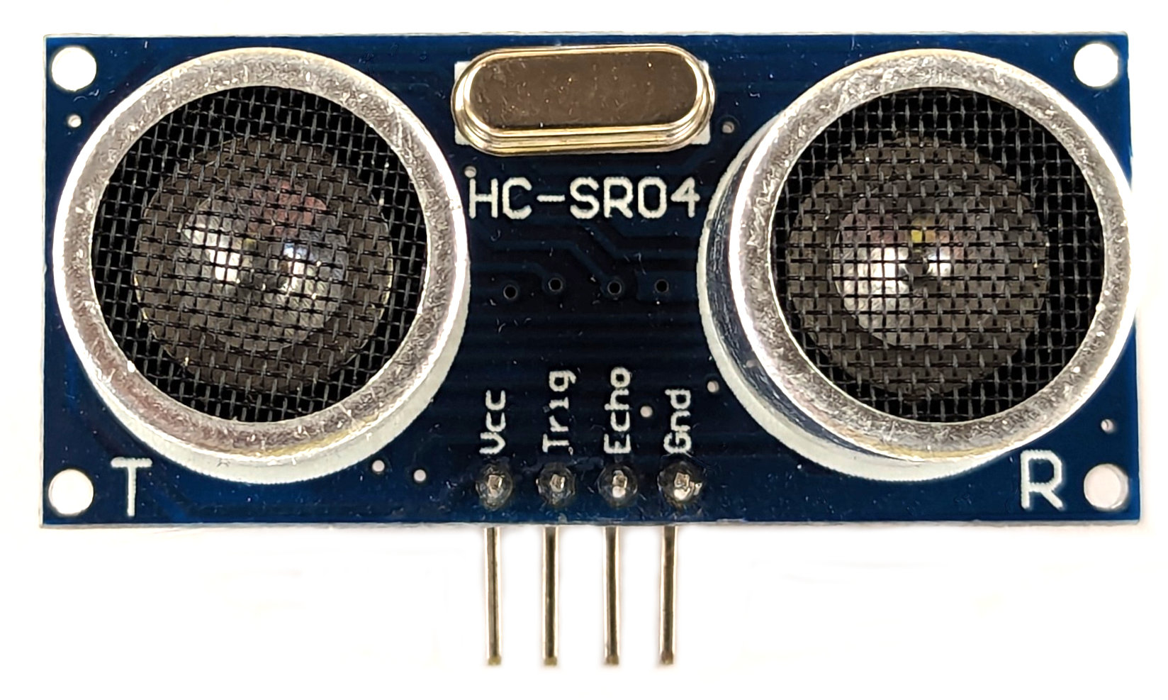
In industry they are widely used for liquid level detection and in cars to sound an alert when you get too close to an object.

How does an Ultrasonic Sensor Work?

Ultrasonic distance sensors use a transmitter to emit high frequency sound. The sound reflects off any object it strikes and returns to a receiver. We can think of the transmitter as a speaker and the receiver as a microphone.

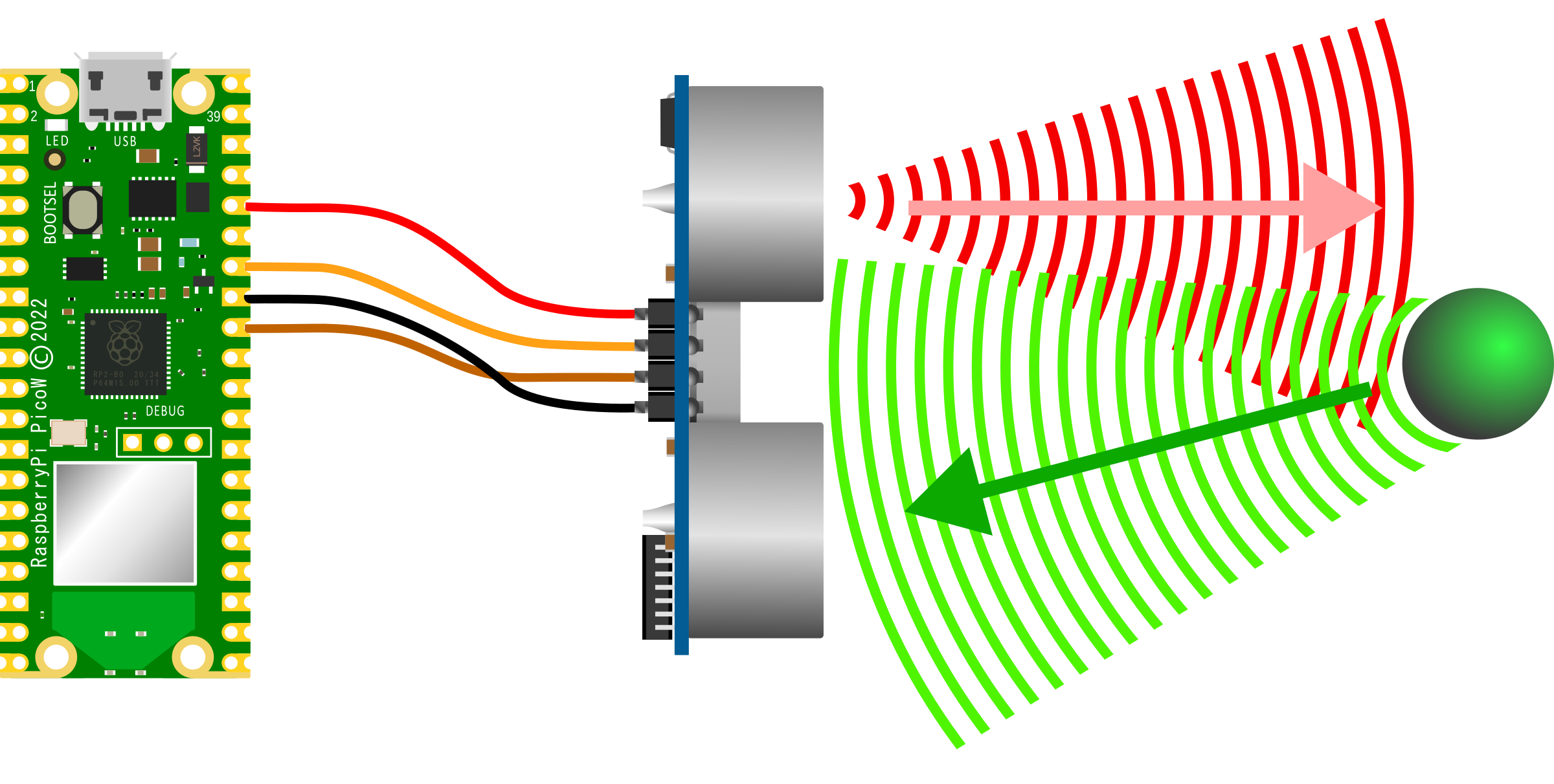
Based on the time difference between the emission of the sound and its return it is able to represent the distance between the object and the sensor.

The sensor we will be using is a HC-SR04P ultrasonic sensor. Be aware that there are two practically identical sensors of this type available. An HC-SR04 and an HC-SR04P The HC-SR04 is designed to work with a 5V supply and to use logic levels that are higher than the compatible input and output from the Pico (although they might work, I wouldn’t recommend it). The connection diagrams shown here are for the simpler HC-SR04P, but we will examine an alternative connection method for an HC-SR04 as well.

This sensor can provide an accurate distance measurement to objects between about 2cm to 4m with a resolution of about 3mm. The sound that is emitted is at 40kHz, and as such well above the limit of human hearing. However, there are a range of animals that could potentially hear a noise at that frequency, including bats, cats, dogs, seals, sea-lions and a range of dolphins and porpoises.

The HC-SR04P uses piezoelectric elements (ultrasonic transducers) in their sensor components. One will transmit a certain frequency of sound (like a speaker) when a signal is applied and the other will generate an electrical output when it receives a sound of a certain frequency (like a microphone).

The HC-SR04P is triggered with an applied signal and a sequence of eight 40kHz pulses are generated by the transmitter.

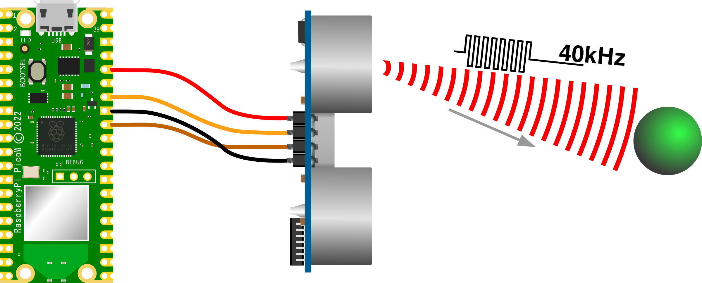
At the same time that the pulses are transmitted, the HC-SR04P’s ‘Echo’ pin is set to high

The pulses are reflected off an object back to the receiver portion of our sensor

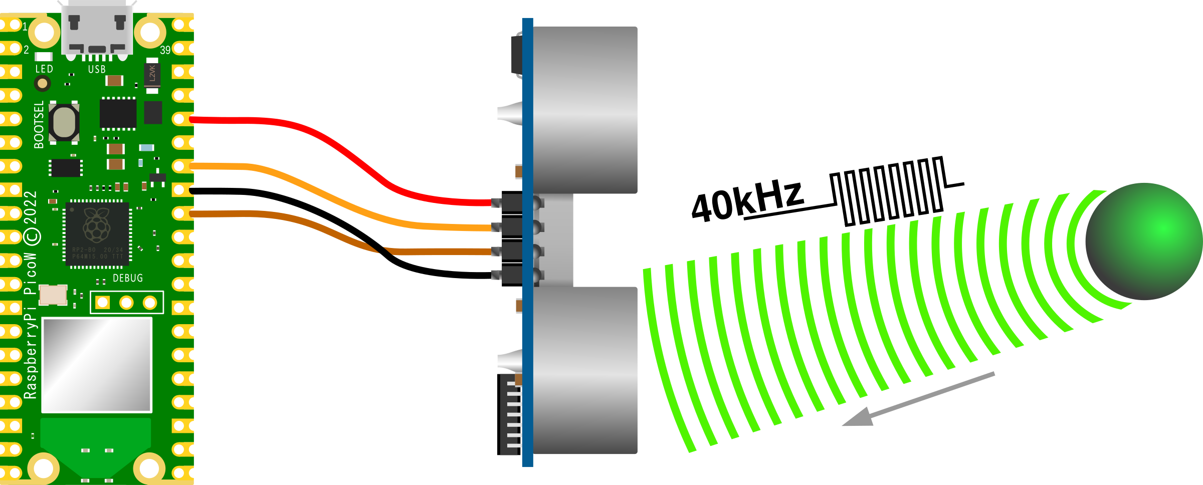
When the receiver collects the pulses, the ‘Echo’ pin is set to low and what we are left with is a pulse from our ‘Echo’ pin which has a width dependant on the distance of the object.

If the pulses don’t get reflected back to our receiver (i.e. there isn’t an object to measure) the ‘Echo’ pin will automatically go low after 38ms.

The time limits for receiving the pulses back are between 150µs and 25ms. These are the bounds for our ‘Echo’ signal. A 150µs ‘Echo’ signal corresponds to 2cm and 25ms is 4m.

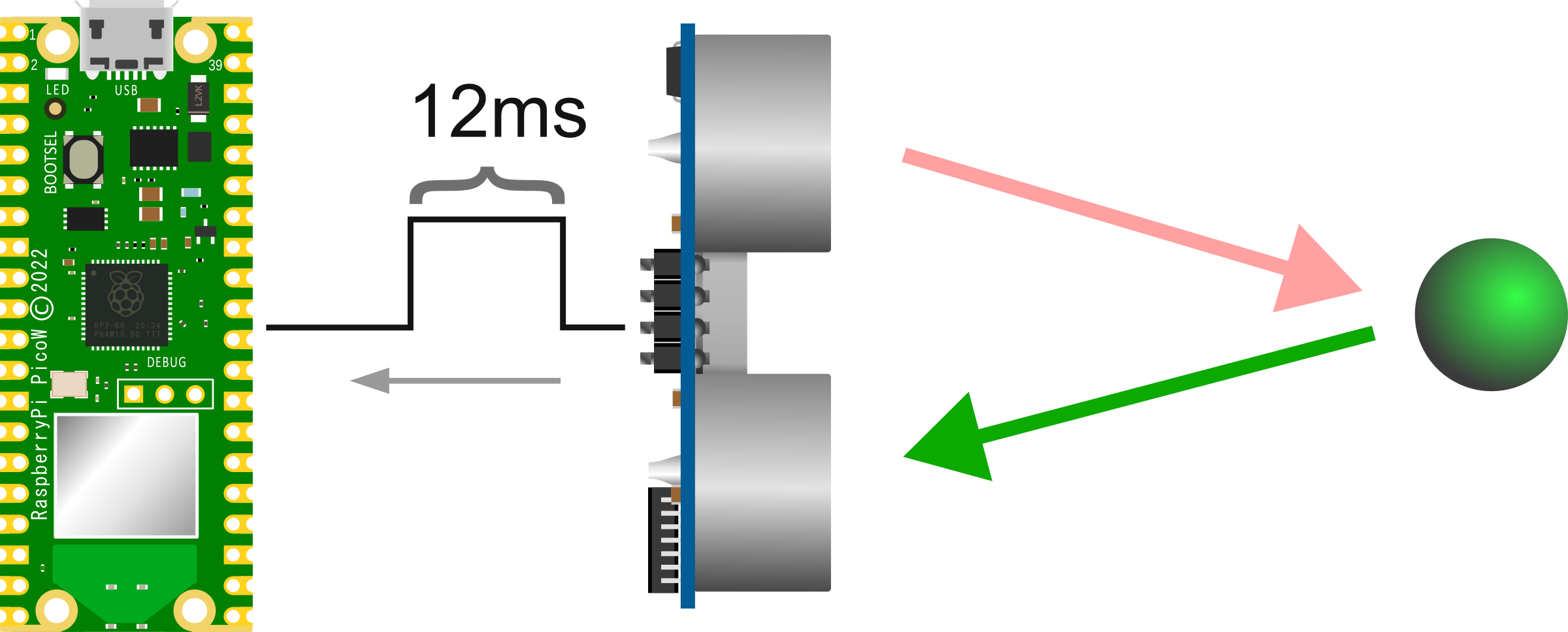
The distance from the sensor to the reflecting object can be found by multiplying the time that the echo pin was high (represented as 12ms in the diagram) by the speed of sound (340m/s) and dividing by 2 (since the sound travelled out and back). Therefore;

Our object is 2.04 metres away!

Connecting an Ultrasonic Sensor Up to the Pico

As mentioned earlier, there are two almost identical models of this particular ultrasonic sensor. The HC-SR04 which works with 5V supply and logic, and the HC-SR04P which will work with supply and logic levels from 3.0V to 5.5V. For the Pico it will be easier to work with the HC-SR04P which will only require four connections. 3.3V power (Vcc), ground (Gnd), Trigger (Trig) and Echo (Echo). The following connections are used for this example;

• HC-SR04 Vcc to the 3V3(OUT) (pin 36) on the Pico (Red)
• HC-SR04 Gnd to Ground (GND) (pin 33) on the Pico (Black)
• HC-SR04 Trig to GP28 (pin 34) on the Pico (Orange)
• HC-SR04 Echo to GP27 (pin 32) on the Pico (Brown)

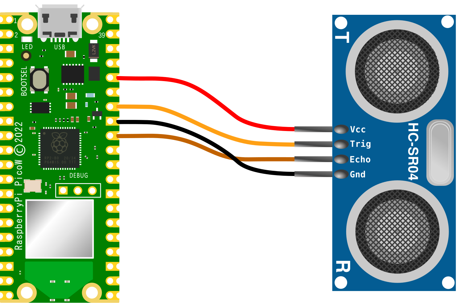
If we wanted to use the 5V supplied HC-SR04 we would want to incorporate a level shifter into the circuit to reduce or increase the signal levels between the devices. The connection would look something like the following;

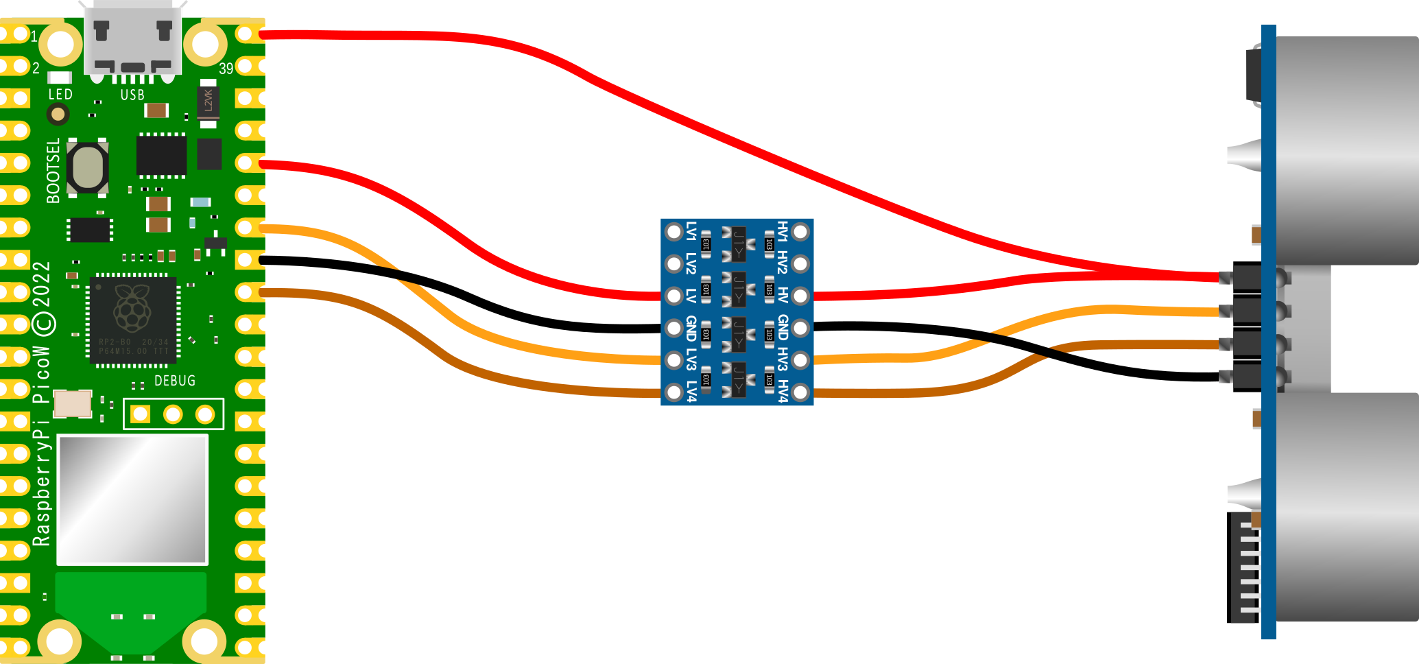
Or for those who prefer a more real-world example…

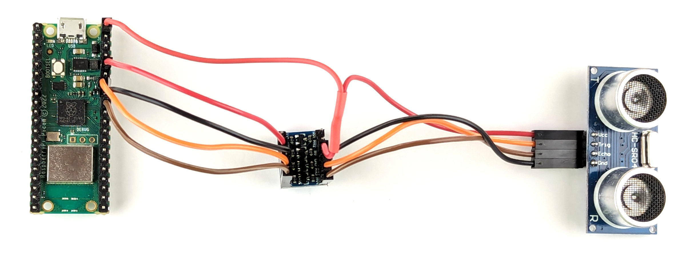
Code

The code below is pretty simple and relies on setting the trigger and echo pins, sending the trigger pulse, measuring the echo pulse and then printing the result.

from machine import Pin
import time

trig=Pin(28, Pin.OUT)
echo=Pin(27, Pin.IN)

while True:
     # Send the trigger
    trig.high()
    time.sleep_us(11)
    trig.low()
    
    #Wait for the echo
    while (echo.value()==0):
        pass
    lastreadtime=time.ticks_us() # record when echo went high
    while (echo.value()==1):
        pass # wait for echo to finish
    echotime=time.ticks_us()-lastreadtime # how long was the echo pulse

    # Print out the distance
    if echotime>37000:
        print("No obstacle in range")
    else:
        distance = (echotime * 0.034) / 2
        print(f"Distance : {distance} cm")
    time.sleep_ms(500)

Reading the on-board Temperature of a Raspberry Pi Pico

As well as providing many marvellous ways of interfacing to the world via external sensors, the Raspberry Pi Pico, or more accurately, the RP2040 microcontroller around which the Pico is built, includes an on-board temperature sensor that we can access to get a feel (see what I did there) for the environment.

About the sensor

As we know from reading about the RP2040 microcontroller, it includes an Analogue to Digital Converter (ADC) which can read signals that vary across a (relatively) broad range of input voltage levels and convert them to discrete values that we can read.

The RP2040 has five ADC inputs. Three are connected to the GPIO pins. One is connected to GPIO29 (which isn’t exposed as a header pin) which is used to measure VSYS and one input is dedicated to an internal temperature sensor. Don’t go trying to look for the sensor on the Pico board, it is integrated into the main RP2040 microcontroller chip!

The ADC on the Pico will allow for 12 bit resolution. That means it will return analogue values to a digital range between 0 and 4095. However, we will be scaling those values to a 16 bit range when we read them with MicroPython to between 0 and 65535. So for us, a voltage range between 0v and 3.3v will equal a digital numeric range of between 0 and 65535.

Technically the temperature of 27°C should equal the voltage of 0.706V which should equal 14021 on our numeric range between 0 and 65535.

As our temperature increases, the voltage reading drops by 1.721mV per degree.

Therefore the logical process that we need to follow to arrive at a temperature is;

1. Read our 16 bit value. (variable = reading)
2. Convert our 16 bit value into the equivalent voltage (variable = voltage) by multiplying our reading by 3.3/65536.
3. Solve for the last unknown which is the variable temperature. Since we know where one point of the linear graph of voltage to temperature is (0.706V at 27°C) and we know the voltage of our ADC input and we know the rate of change (gradient) of our graph (-1.721mv per °C).

Points to note from the datasheet

The rate of change of the sensor can vary over the temperature range and from device to device, therefore some degree of calibration may be required to gain a more accurate measurement.

Likewise, the sensor is very sensitive to errors in the reference voltage. Any error in the reference voltage will be passed to the measurement. The method to improve accuracy is therefore to add a more accurate and stable external reference voltage.

Code

The code below is a very simple affair that declares our sensor then enters a loop where a reading is taken, converted to a voltage, translated to a temperature and printed. This is repeated every two seconds.

import machine
import time

sensor = machine.ADC(4)

while True:
    reading = sensor.read_u16()
    voltage = reading * ( 3.3 / 65535) 
    temperature = 27 - (voltage - 0.706) / 0.001721
    print('Temperature: ', temperature)
    time.sleep(2)

The output can be adjusted by carefully breathing on the Pico which should raise the temperature slightly.

Temperature:  15.3408
Temperature:  14.87265
Temperature:  15.80894
Temperature:  15.3408

It should be noted that the large number of decimal places in the output is not indicative of a commensurate level of accuracy!

Multiple Temperature Measurements

This project will measure the temperature at multiple points using DS18B20 sensors. We will use the waterproof version of the sensors since they are more practical for external applications.

The DS18B20 Sensor

The DS18B20 is a ‘1-Wire’ digital temperature sensor manufactured by Maxim Integrated Products Inc. It provides a 9-bit to 12-bit precision, Celsius temperature measurement and incorporates an alarm function with user-programmable upper and lower trigger points.

Its temperature range is between -55C to 125C and they are accurate to +/- 0.5C between -10C and +85C.

It is called a ‘1-Wire’ device as it can operate over a single wire bus thanks to each sensor having a unique 64-bit serial code that can identify each device.

While the DS18B20 comes in a TO-92 package, it is also available in a waterproof, stainless steel package that is pre-wired and therefore slightly easier to use in conditions that require a degree of protection. The measurement project that we will undertake will use the waterproof version.

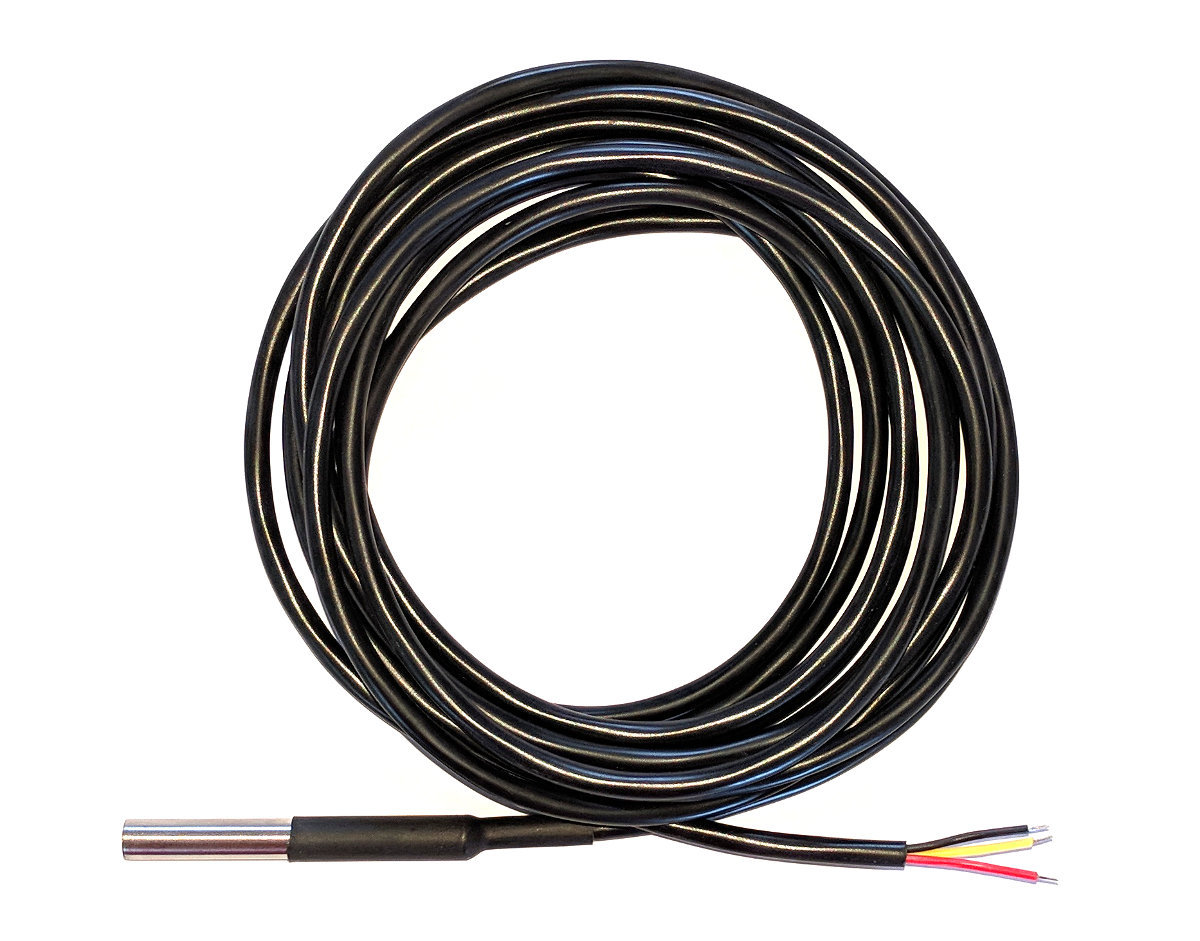
The sensors can come with a couple of different wire colour combinations. They will typically have a black wire that needs to be connected to ground. A red wire that should be connected to a voltage source (in our case a 3.3V pin from the Pico) and a blue or yellow wire that carries the signal.

The DS18B20 can be powered from the signal line, but in our project we will use the supply from the Pico.

Hardware required

• 3 x DS18B20 sensors (the waterproof version)
• 4.7k Ohm resistor (I have used 10k Ohm resistor without problem)
• Jumper cables with Dupont connectors on the end
• Solder
• Heat-shrink

Connecting everything up

The DS18B20 sensors needs to be connected with the black wires to ground, the red wires to the 3V3 pin and the blue or yellow (some sensors have blue and some have yellow) wires to GP26 (pin 31). A resistor between the value of 4.7k Ohms to 10k Ohms needs to be connected between the 3V3 and GP26 pins to act as a ‘pull-up’ resistor.

We can actually use any of our GP pins to connect our sensors, as our code will will rely on a software library to manage the communications, not one of the hardware implementations on the microcontroller.

The following diagram is a simplified view of the connection.

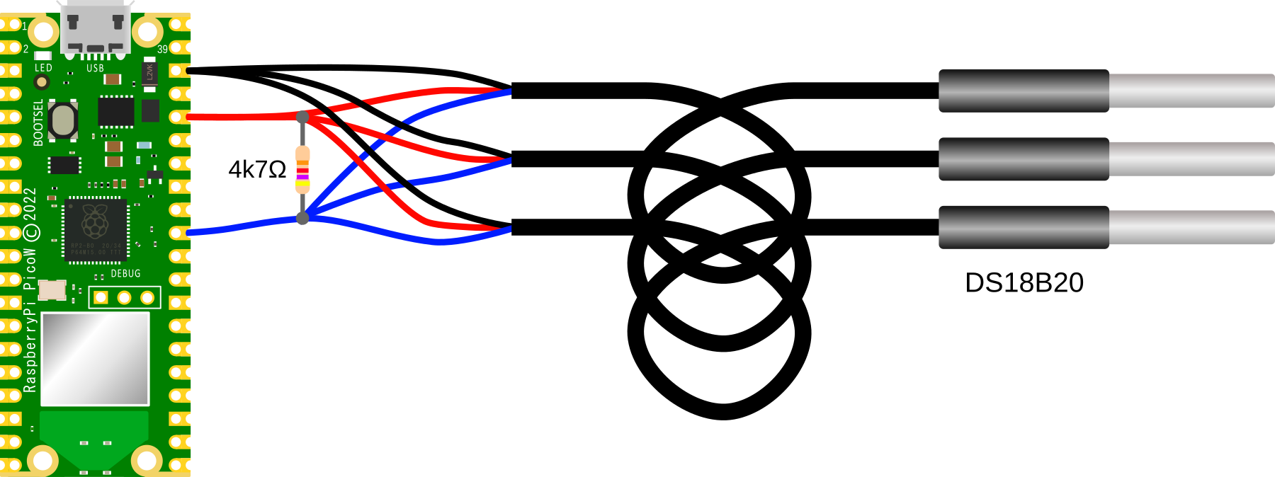
Connecting the sensor practically can be achieved in a number of ways. But because the connection is relatively simple we can build a minimal configuration that will plug directly onto the appropriate GPIO pins using Dupont connectors. The resistor is concealed under the heat-shrink and indicated with the arrow.

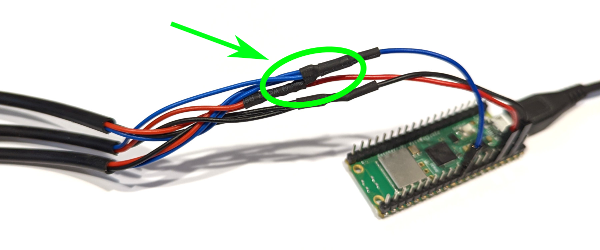
Code

The following code will read the temperature values from all the DS18B20 sensors that it finds and print out the unique serial numbers of each sensor and the temperature that it is reading.

import machine
import onewire
import ds18x20
import time
import binascii

gp_pin = machine.Pin(26)

ds18b20_sensor = ds18x20.DS18X20(onewire.OneWire(gp_pin))

sensors = ds18b20_sensor.scan()

print('Found devices: ', sensors)

while True:
    ds18b20_sensor.convert_temp()
    time.sleep_ms(750)
    for device in sensors:
        s = binascii.hexlify(device)
        readable_string = s.decode('ascii')
        print(readable_string)
        print(ds18b20_sensor.read_temp(device))
    time.sleep(10)

The output will look something like the following (which has three sensors connected);

Found devices:  [bytearray(b'(\xff\xef\x8d>\x04\x00\xa8'), bytearray(b'(\xffI\x90\
>\x04\x00\xa2'), bytearray(b'(\xff\xf8n;\x04\x00q')]
28ffef8d3e0400a8
19.8125
28ff49903e0400a2
20.4375
28fff86e3b040071
19.625

AHT10 Temperature and Relative Humidity

It is quite common to package multiple sensors into a single package and the AHT10 is a good example that measures temperature and relative humidity.

AHT10 Details

The AHT10 is an accurate temperature and humidity sensor in a very small package that can be accessed via an I2C interface. While it has a temperature measurement range of between -40°C and 85°C, its typical error of ± 0.3 is achieved between around 0°C and 55°C. Normal operating range for humidity is between 20 and 80% relative humidity. In that range it has a typical accuracy of ±2.

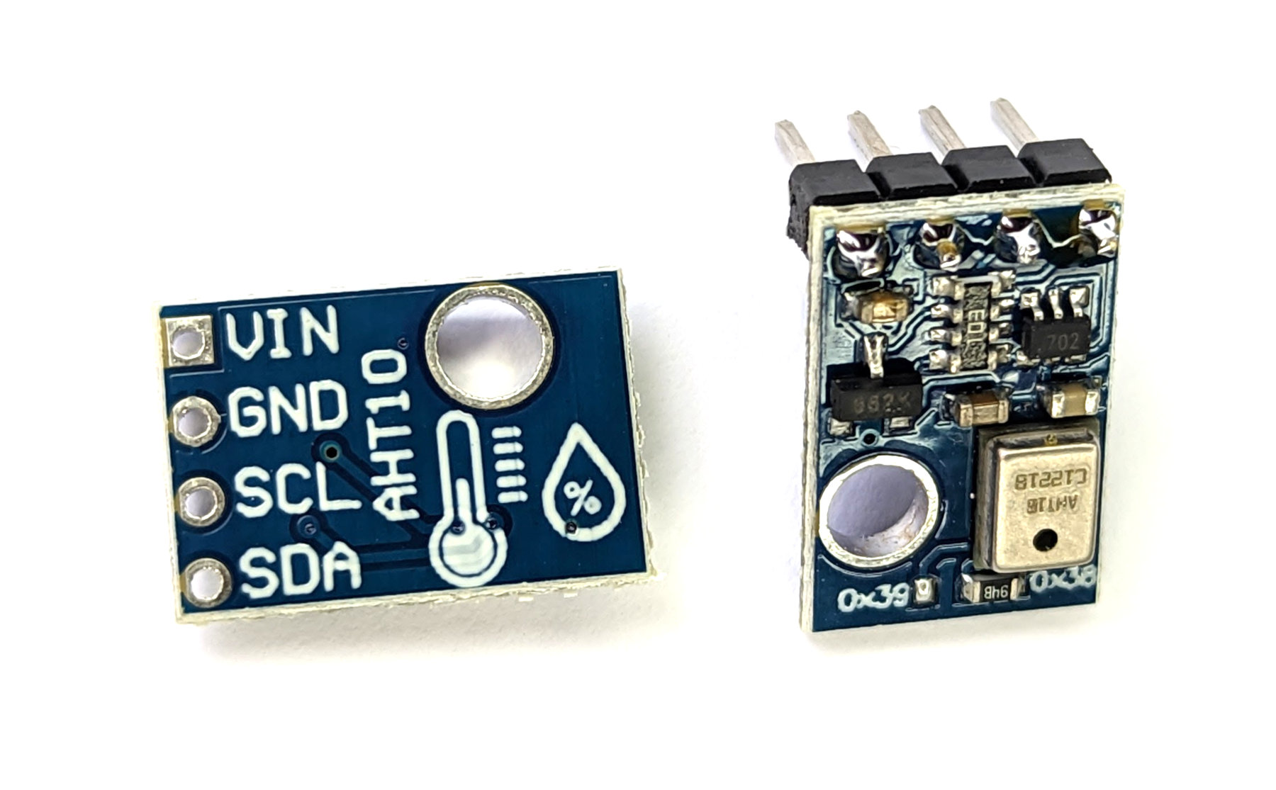
Each sensor is calibrated and tested with a product lot number printed on the surface. be aware that humidity sensors are not ordinary electronic components and should be carefully handled and operated. Prolonged exposure to high concentrations of chemical vapour will cause the sensor reading to drift.

If the sensor is exposed to adverse conditions or chemical vapours and the readings drift, it can be restored to its calibrated state by the following process;

• Drying: maintained at 80-85 ° C and <5% relative humidity for 10 hours;
• Rehydration: 12 hours at 20-30 ° C and >75% relative humidity.

The devices address is 0x38 (which we will see when we scan it) and in spite of there also being the address 0x39 also printed on the sensor PCB, there is no indication of how to enable that address. As a result, only a single AHT10 can be used on an I2C bus.

How is the AHT10 sensor accessed?

The sensor is accessed via I2C, but we can abstract the complexities of this via a pre-built MicroPython module. This was developed by Andreas Bühl. To make use of the module we will need to download it from GitHub and then copy it over to our Pico. I found this most easily accomplished by first downloading the file to the main computer and then going File >> Open on Thonny and selecting the appropriate file. From there go File >> Save as… and select the Pico as the location to save the file (making sure to save it with the appropriate name (ahtx0.py))

Because of the abstraction afforded by the library, the reading of the sensor is nicely simplified.

Connecting the AHT10 to the Pico

The connection is fairly simple with only four connections being required. Power, ground, Serial CLock line (SCL) and Serial DAta line (SDA). The following connections are used for this example;

• AHT10 GND to Ground (pin 38) on the Pico (Black)
• AHT10 VIN to the 3V3(OUT) (pin 36) on the Pico (Red)
• AHT10 SCL to I2C1 SCL (pin 32, or GPIO27) on the Pico (Orange)
• AHT10 SDA to I2C1 SDA (pin 31, or GPIO26) on the Pico (Brown)

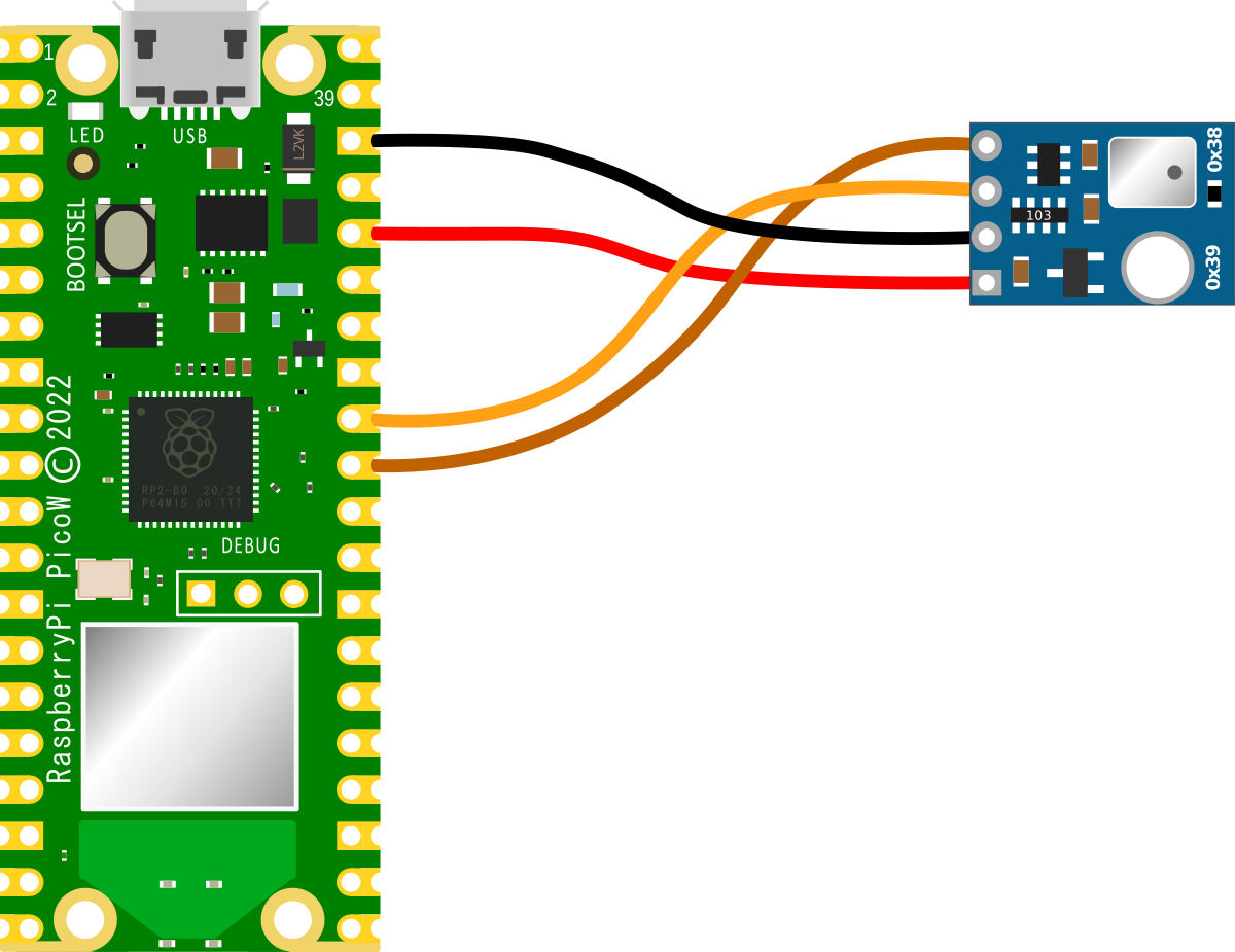
Assuming that we have header pins soldered onto our Pico and the AHT10 sensor, the easiest ways to make a connection is via Dupont connectors.

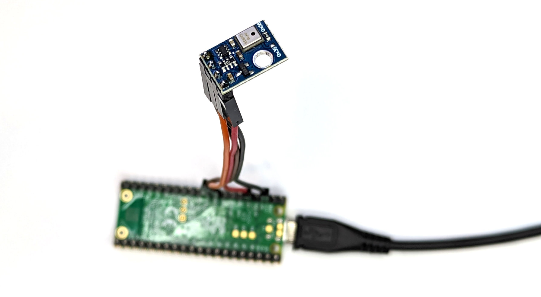
An important point to note when we are connecting our Pico is that because the RP2040 microcontroller has two I2C controllers we need to ensure that we define which controller we are using in the code. I2C0 = id 0 and I2C1 = id 1. This is set in the following lines in the MicroPython code;

i2c = I2C(1, sda=sda, scl=scl)

Code

As a neat method of confirming the address of our sensor we can run the following code on our Pico that will scan the I2C bus;

from machine import Pin, I2C

# Create I2C object
sda = Pin(26)
scl = Pin(27)
i2c = I2C(1, scl=scl, sda=sda)

# Print out any addresses found
devices = i2c.scan()

if devices:
    for d in devices:
        print(hex(d))

This will print out;

0x38

Which is the address printed on the circuit board.

The code to measure the temperature and relative humidity is;

import time
from machine import Pin, I2C

import ahtx0

# Create I2C object
sda = Pin(26)
scl = Pin(27)
i2c = I2C(1, scl=scl, sda=sda)

# Create the sensor object using I2C
sensor = ahtx0.AHT10(i2c)

temperature = round(sensor.temperature, 2)
humidity = round(sensor.relative_humidity, 2)

while True:
    print("Temperature: ", temperature, "C")
    print("Humidity: ", humidity, "%")
    print()
    time.sleep(5)

Just a reminder that if we use different I2C pin than GPIO26 and GPIO27, we will need to check the pinout to know which I2C id should be used. In the case above it is 1.

Which produces something like the following;

Temperature:  21.98 C
Humidity:  55.41 %

Temperature:  21.98 C
Humidity:  55.41 %

Temperature:  21.98 C
Humidity:  55.41 %

To see some variation, we can softly breath on the sensor.

Motion Sensing with the Raspberry Pi Pico

What is a PIR Sensor?

A passive infrared (PIR) sensor measures and evaluates InfraRed (IR) light emitted from nearby objects. They are referred to as ‘passive’ due to the fact that the sensor does not emit any heat or energy. Living animals emit infrared radiation and the sensor can pick this up and register it electronically. It uses a clever mechanism to detect a change in the infrared light it is receiving and as a result trigger a signal that can be read by an external device. In our case that will be a Raspberry Pi Pico.

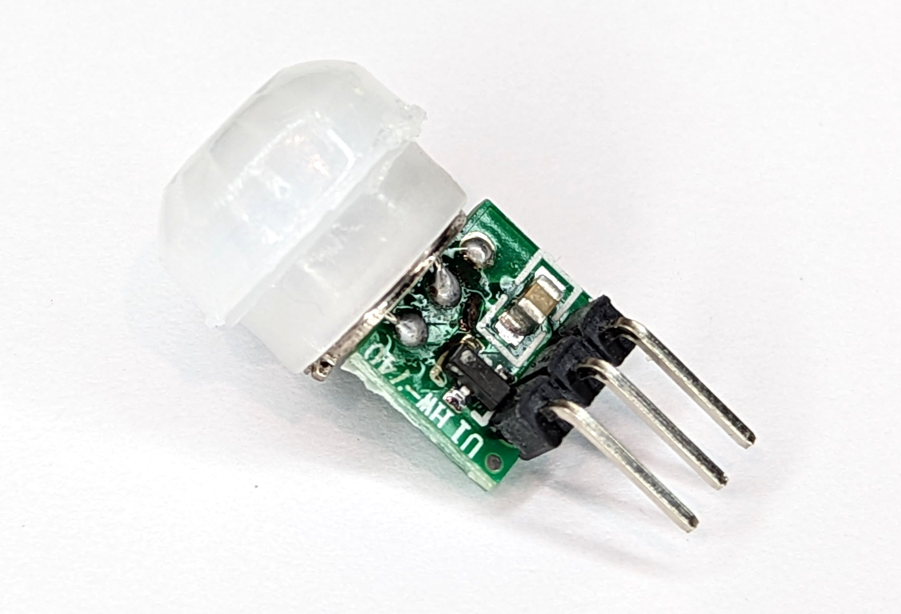
PIR sensors are used in sensing applications, such as security alarms, motion detectors, and automatic lights.

How does a PIR Sensor Work?

Pretty much everything (humans, animals, even inanimate objects) emit a certain amount of infrared radiation. The amount relates to the body or object’s warmth and composition.

The PIR sensor proper is actually under the white hemispherical covering that is prominent on a PIR. The covering is in fact a lens that focusses radiation onto the sensor. The sensor has two slots in it where each slot allows infrared radiation to interact with pyroelectric receptors that are very sensitive to this type of emission at room temperature. The sensor is a hermetically sealed metal enclosure which improves immunity to noise, temperature and humidity. The sensor incorporates a window made of infrared-transmissive material for protection.

When there is no warm moving object in the sensors field of view it is idle and both slots detect the same amount of radiation. However, when a warm body like a human or animal comes into view, a signal is first detected by one of the pyroelectric sensors, which causes a positive differential change between the two halves. When the warm body leaves the sensing area, the reverse happens and the sensor generates a negative differential change. These changing pulses are what determines that movement has been detected.

The PIR sensor is mounted on a printed circuit board which supports the electronics that interpret the signals from the sensor itself. In a practical setting the complete assembly is usually contained within a housing which is located to provide a view over the area to be monitored.

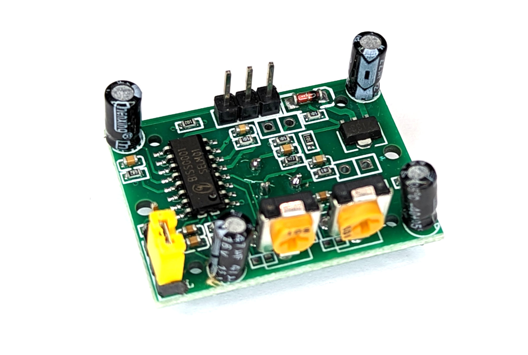
The white hemispherical lens is essentially a ‘window’ through which the infrared energy can enter. The plastic lens acts as a focusing mechanism which condenses a large area into a small one (in the same way that a camera lens works). To minimise the cost and size required the covering is normally a fresnel lens.

The HC-SR501

I’m including the HC-SR501 description here because I have a few hanging around and I had great plans to use one for a particular project involving a Raspberry Pi Zero some months ago. However, in the process of testing I found that it would trigger at times through interference with the WiFi signal on the Pi. This took quite a period to determine as I went through troubleshooting which included multiple sensors and different Pis. Ultimately I came to the conclusion that the analog portion of the design of the HC-SR501 that allowed the device to trigger unintentionally was not suitable for my application and I used the AM312 instead. That device uses digital signal processing which was unaffected by the WiFi signal.

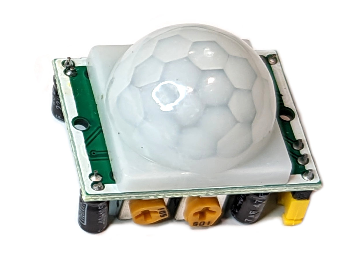
The HC-SR501 has a 3-pin connector that interfaces it to the outside world. The connections are as follows;

• VCC is the power supply for HC-SR501 PIR sensor which we can connect a 5V pin.
• Output pin is a 3.3V TTL logic output. LOW indicates no motion is detected, HIGH means some motion has been detected.
• GND should be connected to the ground.

The HC-SR501 has a built-in voltage regulator so it can be powered by any DC voltage from 4.5 to 12 volts, typically 5V is used.

There are more than one model of this type of sensor. be careful to ensure that you have the connections correct. The best mechanism (other than following the labels if there are any) is to look for the protection diode as a reference. Failing that, if there aren’t any labels on the bottom of the circuit board, check on the board, under the lens.

There are two potentiometers on the board to adjust a couple of parameters;

• Sensitivity: This sets the maximum distance that motion can be detected. It ranges from 3 meters to approximately 7 meters. The layout of the area being covered can affect the range.
• Time: This sets how long that the output will remain high after detection is triggered. The minimum is 3 seconds and the maximum is 300 seconds or 5 minutes.

The board also has a jumper with two settings;

• H: This is the Hold / Repeat / Retriggering setting. In this position the HC-SR501 will continue to generate a high output while it continues to detect movement.
• L: This is the Intermittent or No-Repeat / Non-Retriggering setting. Here the output will stay high for the period set by the Time potentiometer.

As with most PIR sensors the HC-SR501 requires some time to adjust to the infrared environment that it sees in any room. This will take from 30 to 60 seconds when the sensor is first powered up. It also has a ‘reset’ period of about 5 or 6 seconds after making a reading. During this time it will not detect any motion.

The AM312

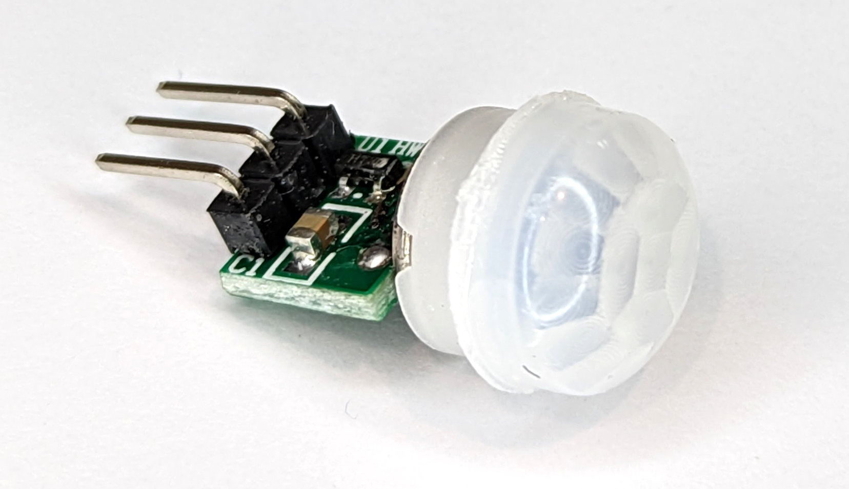
As mentioned earlier, the AM312 utilises digital signal processing which removes one of the reasons that interference can affect the HC-SR501.

AM312 is described as a new digital intelligent PIR sensor! It is a much simpler and smaller device than the HC-SR501 with the digital detector and electronic circuitry built into the detector housing.

This sensor also has the advantage of being ultra-low power with a quiescent current of only 8uA making it suitable for battery applications where a very long battery life is required.

The pin connections are as follows with the orientation of the sensor with the header pins uppermost;

• Vin is the power supply which requires 3.3VDC.
• The Signal pin will present a high when motion is detected.
• Ground should be connected to the ground.

How do we read a PIR?

A PIR is one of the simplest sensors to read with the signal pin going high when motion is detected. This means that we can merely set any one of our GPIO pins to act as an input and then read when it goes high.

Connecting Up a PIR to the Pico

For the AM312 we can connect the sensor to the Pico as follows;

- Vin on the AM312 to the 3V3(Out) pin (36) on the Pico.
- Signal pin on the AM312 to GPIO 28 (pin 34) on the Pico.
- Ground should be connected to the GND pin (38) on the Pico

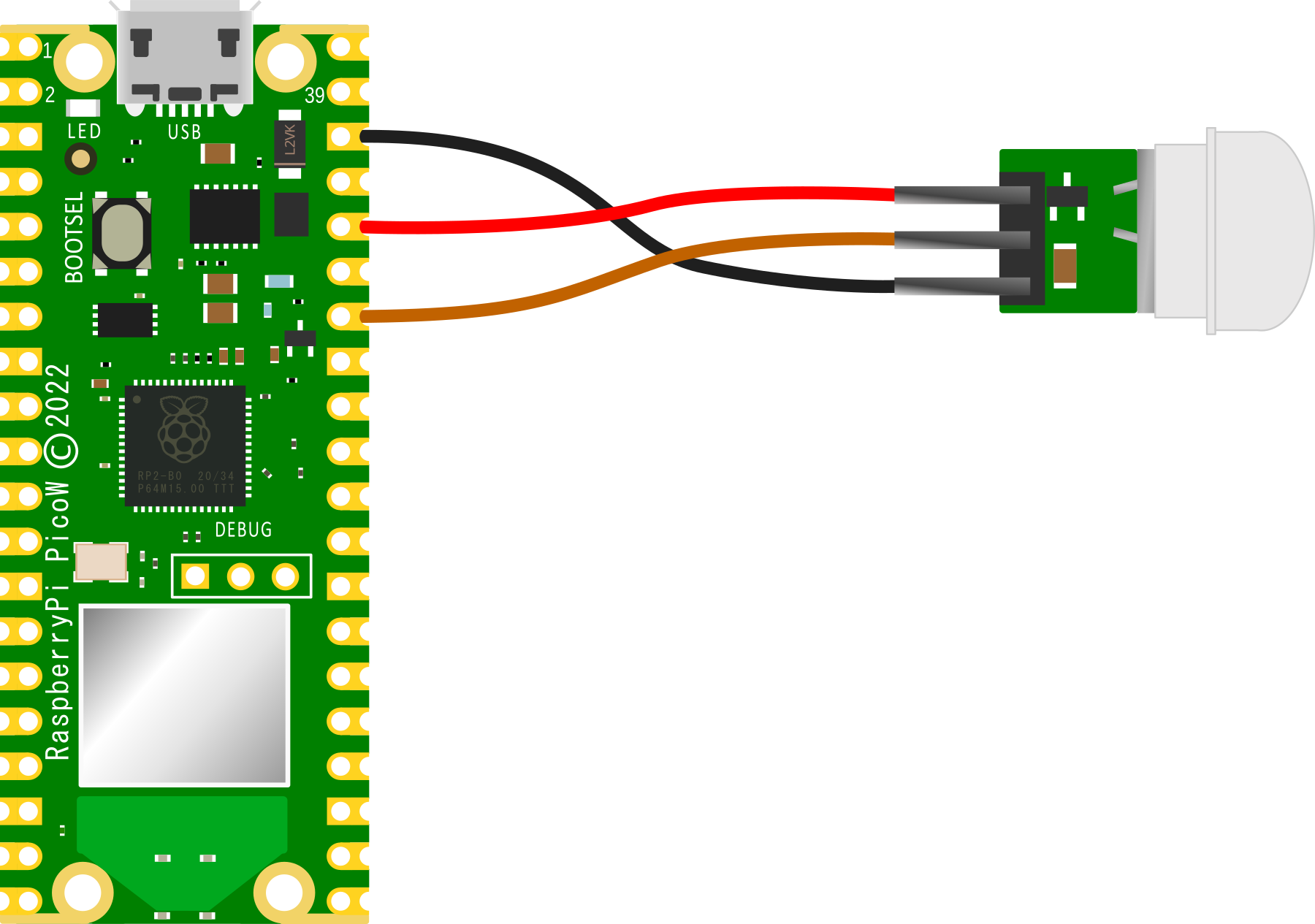
Connecting the PIR practically can be achieved in a number of ways. But because the connection is relatively simple we can build a minimal configuration that will plug directly onto the pins using Dupont header connectors and jumper wire.

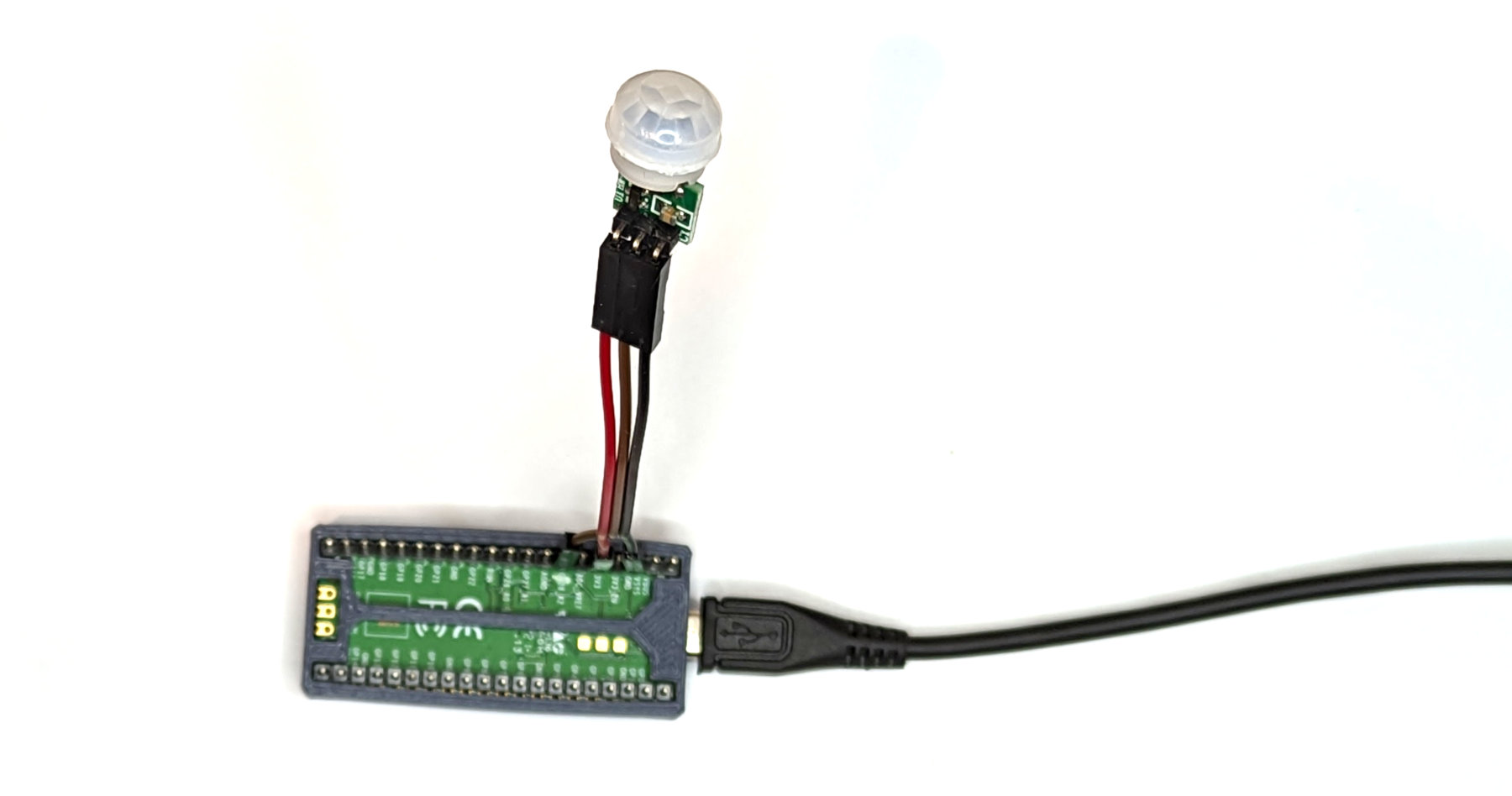
Be aware that there are a few similar models of this type of sensor. Be careful to ensure that you have the connections correct. The best mechanism (other than following the labels if there are any) is to look for the protection diode as a reference on the HC-SR501 and be aware that the diagram that I have shown here for the AM312 is shown with the header pins uppermost. For example the sensor I am using is not labelled, and the VCC and GND pins are in a different location to those shone on at least one connection diagram on the Internet.

Code

The code below will designate the GPIO pin to be used as our input (GPIO28) and set it low with a pull down resistor.

pir = Pin(28, Pin.IN, Pin.PULL_DOWN)

We can use any of the GPIO pins, so feel free to pick a convenient one. We use an internal pull down resistor to avoid having a ‘floating’ input. This will set the pin to be a logic 0 so long as it doesn’t have a signal applied.

It pauses momentarily to gather itself and then goes into an eternal loop where it prints out an alert when movement is detected. It also pauses after detection to give the detectors signal output an opportunity to return to a low state.

import time
from machine import Pin

pir = Pin(28, Pin.IN, Pin.PULL_DOWN)
count = 0

time.sleep(1)
print('Ready to detect movement!')

while True:
     if pir.value() == 1:
          count = count + 1
          print('Movement detected ', count)
          time.sleep(4)
     time.sleep(1)

Motion detection using a Microwave Doppler Sensor

What is a Doppler Sensor?

A Doppler sensor is a device that transmits a high frequency RF signal and listens for the reflected signal that bounces off nearby objects. That reflected signal will vary in frequency from the transmitted signal if the object it bounces off is moving. This is due to the Doppler effect. The sensor detects the difference in the frequency of the transmitted and reflected signal and produces an output signal when the amount of movement exceeds a specific threshold.

The Doppler Effect

The Doppler effect is named after Christian Doppler who was an Austrian physicist that described the effect in the 1800s. The most common example that most people have experienced is when a car or a train sounding its horn moves towards and then past us. While the car/train is moving towards us the pitch of the horn is high and as it passes us the pitch changes to a lower tone.

Of course some will instantly recognise the effect from the costume worn by Jim Parsons as the character ‘Sheldon Cooper’ in the episode of CBS’s comedy, ‘The Big Bang Theory’ titled ‘The Middle Earth Paradigm’.

This is also the technique used by police forces to determine the speed of motorists on the road. A speed camera or ‘radar gun’ emits a specific Radio Frequency (RF) and since the Doppler effect will make any reflected frequency lower if the car is moving away from the speed camera or higher if the car is moving towards the speed camera, measuring the frequency difference between the emitted signal and the reflected signal can determine the speed of the vehicle.

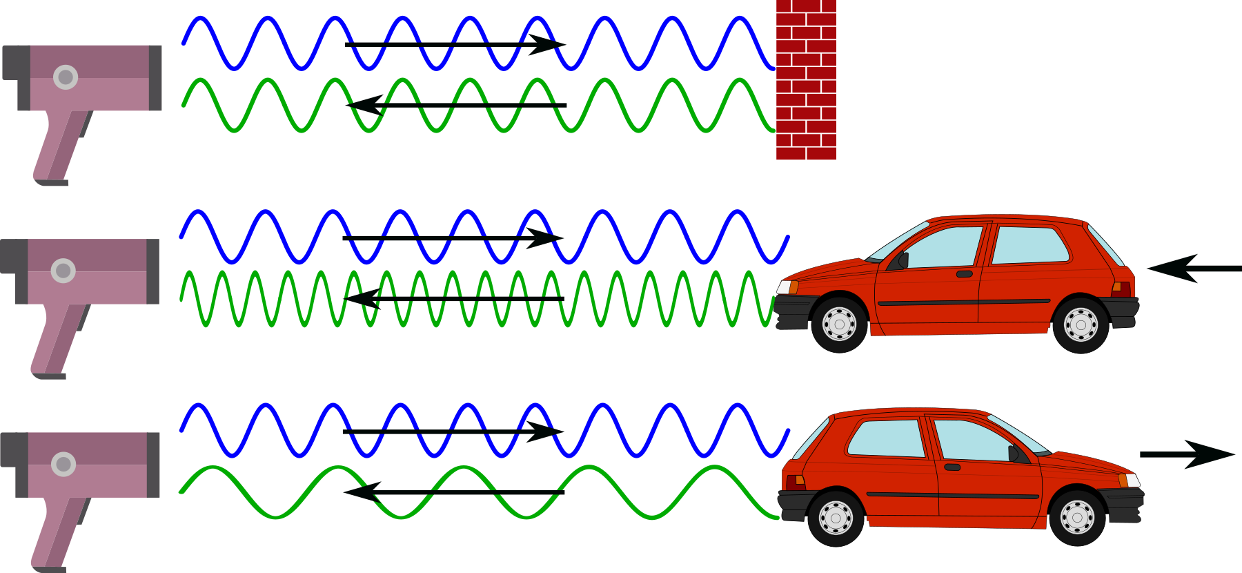
How does a Microwave Doppler Sensor Work?

A microwave Doppler sensor starts with an electronic device called an ‘oscillator’. This device will set the frequency of operation for the unit and allows the transmitter to broadcast a specific frequency from a built in transmitting / receiving antenna. Once broadcast, the signals reflect off the surroundings and are then returned to the sensor and collected by a receiver on the board. This reflected signal will vary in frequency (according to the Doppler effect) if any of the objects that the signal bounced off were moving towards or away from the transmitter. This received signal is then mixed with the original oscillator frequency. The mixing process will produce a difference frequency that is the difference between the original oscillator and the reflected signals.

So when our sensor sees a difference frequency of significant strength, it knows that there has been something moving close by and can generate a signal to represent it.

The RWCL-0516 Microwave Radar Sensor

The sensor that we will use is a very simple device that can take an input voltage of between 4 and 28V. With this it will generate a frequency using an oscillator of around 3.182GHz. The oscillator includes an inductor and capacitor that are formed by the copper etched into the board itself. We can see these as the concentric circles on one side and the ‘S’ shape on the other.

The transmitted frequency is not particularly directional, so anything moving around the unit out to a maximum distance of between 5 to 7 meters can be detected. In fact, because the signal is high enough, it will pass through some semi-solid objects (such as a covering container).

Once movement has been detected an output pin is set to ‘high’ for 2 seconds to identify that there has been a trigger.

The RWCL-0516 has five pins as follows

• 3v3 - This is a 3.3v output that can be used for powering other devices (Just to be clear. This is NOT the connection point to power the RWCL-0516).
• GND - The ground reference point
• OUT - This is the output pin that will indicate movement when it occurs.
• VIN - This is where our input voltage is applied (between 4 to 28V).
• CDS - This pin will allow us to disable an optional light sensor on the board (we won’t be fitting this in our example)

The board also has the provision to add components that can adjust the function of the unit.

• On the front side of the board (the side with the majority of the components) there is a space labelled CDS. This is short for ‘Cadmium DiSulphide’. This is the location where a Light Dependant Resister (LDR) can be added to disable the board when there is sufficient light.

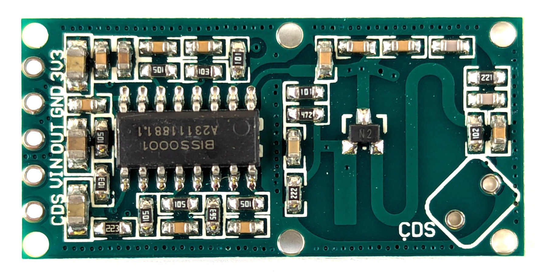
On the rear of the board there are three places that are set aside and labelled to accept components. Be aware that all three will require soldering surface mount devices which will take some considerable care if you haven’t tried it before.

• C-TM - This is a space for a capacitor that adjust the time that the device will stay triggered for once it is set. By default is 2 seconds. A description of values that can be used to extend the time is available from Instructables.
• R-GN - This component change will adjust the detection range. The default is 7m. If we add a 1M resistor here it will reduce to 5m.
• R-RDS - Adding a resistor here will will decrease the effective resistance in series with Light Dependant Resistor (assuming we have it fitted) which lowers the threshold for it to disable the device when it gets brighter. The TLDR explanation (pun intended) is that (assuming you have a LDR fitted in the CDS position) if you put a resister here, the LDR will disable the device at a lower light level.

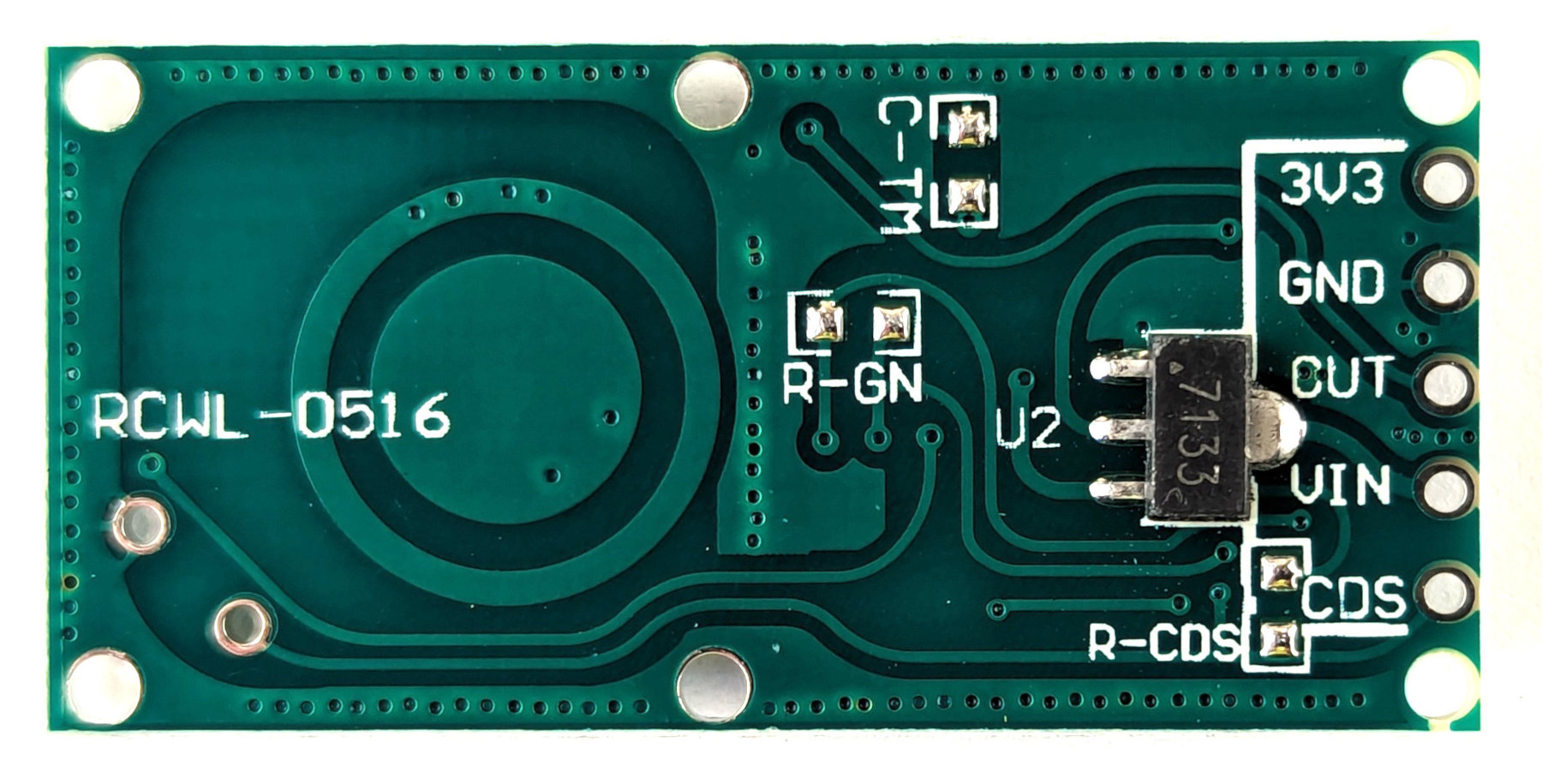
A good deal of information on the unit can be found on the excellent GitHub page maintained by Joe Desbonnet here.

Connecting the RWCL-0516 Sensor Up to the Pico

Our connections can be kept pretty simple. We are going to connect power to the sensor and a signal connection that will indicate when it has been triggered.

• RWCL-0516 VIN to VBUS (pin 40) on the Pico (Red)
• RWCL-0516 GND to GND (pin 38) on the Pico (Black)
• RWCL-0516 OUT to GP28 (pin 34) on the Pico (Orange)

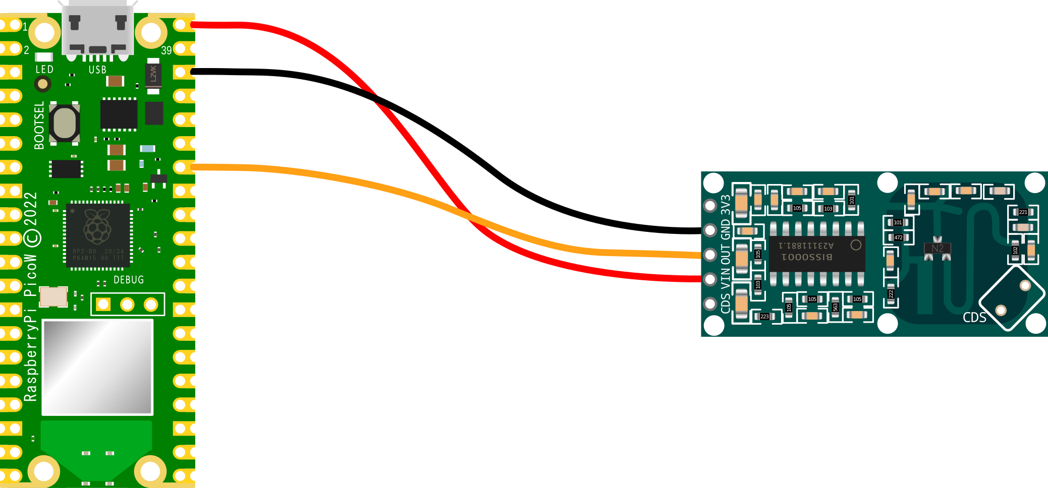
Of course we can simply use our favourite dupont connectors to do the job in the real world.

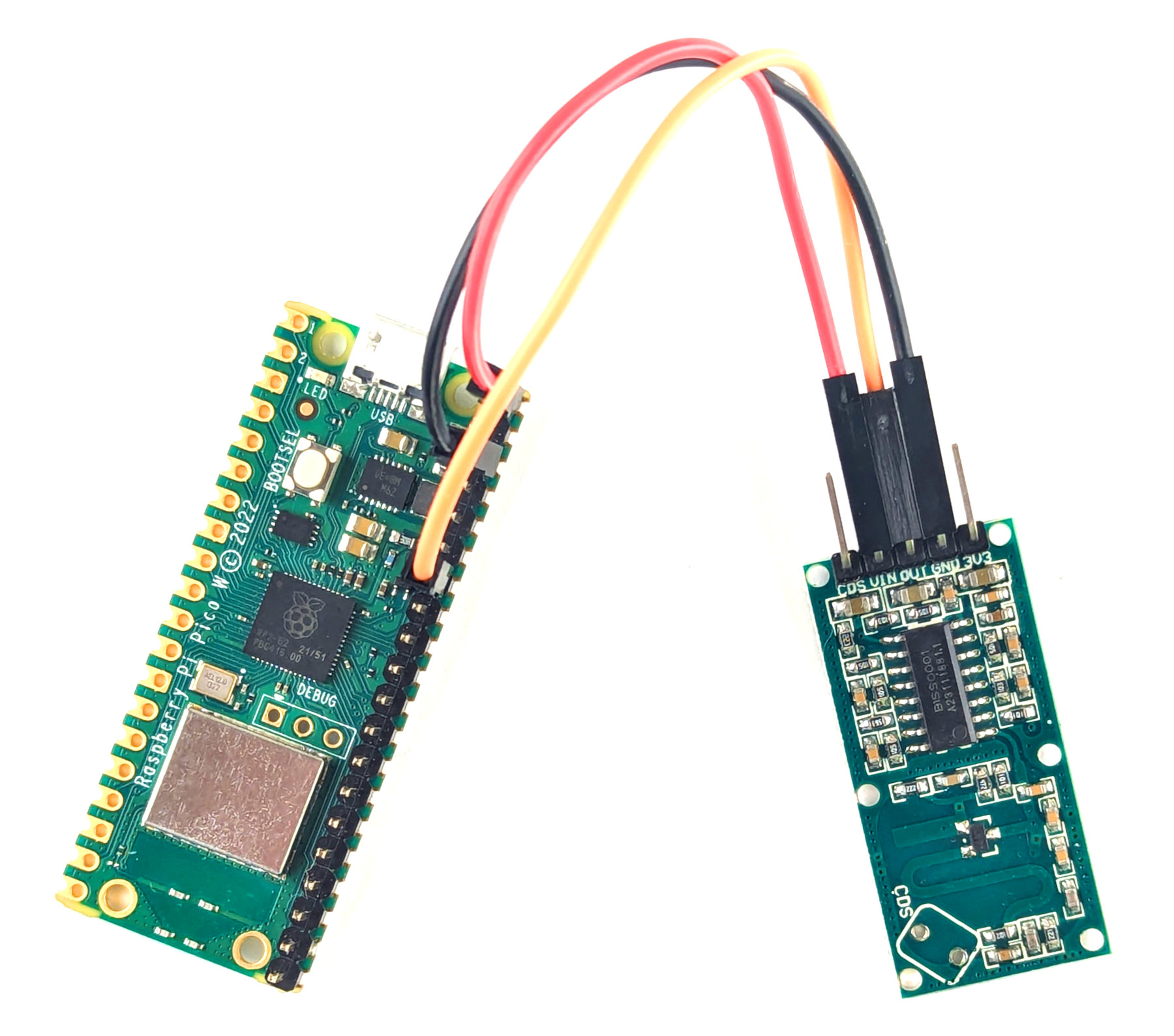
Code

The code below designates GP28 as the pin that the sensor’s out pin is connected to.

It defines a small function to blink the on-board LED and then two functions to operate if the sensor sees motion (it’s blinking time and printing out a notification) or if the environment around it is still.

import time
import machine

motion = machine.Pin(28,machine.Pin.IN)

# Define blinking function for onboard LED    
def blink_onboard_led(num_blinks):
    led = machine.Pin('LED', machine.Pin.OUT)
    for i in range(num_blinks):
        led.on()
        time.sleep(.2)
        led.off()
        time.sleep(.2)

# What to do if motion detected
def moving():
    print("Motion detected")
    blink_onboard_led(1)

# What to do once motion ceased
def still():
    print("Everything is still")

while True:
    if motion.value():
        moving()
    else:
        still()
    time.sleep(1)

It really is a remarkably simple piece of code that we could add to as we wished to carry out other functions if it senses motion.

Sensing vibration with a Raspberry Pi Pico

Vibration sensors

Vibration sensors are designed to convert mechanical movement into a signal that can be measured.

The underlying principles behind vibration sensors vary depending on the type of sensor, but they generally rely on the conversion of mechanical energy (vibrations) into some other form of energy that can be measured and analysed. The most common types of vibration sensors are based on the following principles:

• Piezoelectricity: Piezoelectric sensors rely on the effect which occurs when certain materials, such as quartz, generate an electrical charge in response to applied mechanical stress.
• Capacitance: Accelerometers and displacement sensors often use the principle of capacitance, where changes in the capacitance between two electrodes is proportional to changes in the distance between the electrodes. When the sensor is subjected to a vibration, the distance between the electrodes changes, and this change in distance can be used to measure the vibration.
• Inductance: Inductive sensors measure the change in inductance in a coil caused by the movement of a ferromagnetic core inside the coil. When the ferromagnetic core is subjected to a vibration, the inductance changes, and this change can be used to measure the vibration.
• Magnetic field: Magnetic sensors work when changes in a magnetic field is generated by the movement of a ferromagnetic material inside a sensor.
• Light: Optical sensors use the principle of light and optics, where changes in the light that is transmitted or reflected through the sensor are proportional to changes in the position of a reflecting surface inside the sensor.

In each of these cases, the output signal from the sensor is proportional to the vibration being measured, and the signal can be analysed to determine the frequency, amplitude, and other characteristics of the vibration.

There are several types of movement that vibration sensors can be measure including:

• Acceleration
• Velocity
• Displacement

Each type of vibration sensor has its own strengths and weaknesses, and the choice of sensor will depend on the specific application, including the type of vibration to be measured, the frequency range and the operating environment.

Piezoelectric vibration sensor

A piezoelectric vibration sensor works by converting mechanical energy (vibrations) into electrical energy. The sensor is made up of a piezoelectric material, such as quartz, which has the ability to generate an electrical charge when subjected to mechanical stress.

When a vibration is applied to the piezoelectric sensor, the piezoelectric material deforms and generates an electrical charge proportional to the magnitude of the vibration. This electrical charge can be measured and used to determine the frequency and amplitude of the vibration.

The piezoelectric sensor can be used in a wide range of applications, including measuring vibrations in machinery, detecting structural movements in buildings, and measuring the impact of shock or drop events. The sensors can also be used to monitor and control the vibrations of musical instruments or in anti-tampering systems.

Piezoelectric sensors are generally rugged, reliable, and highly sensitive, making them a popular choice for many applications that require the measurement of vibration or impact

The unit that we will test comes in two parts. There is an interface board which incorporates two screw terminals which attach to the sensor proper.

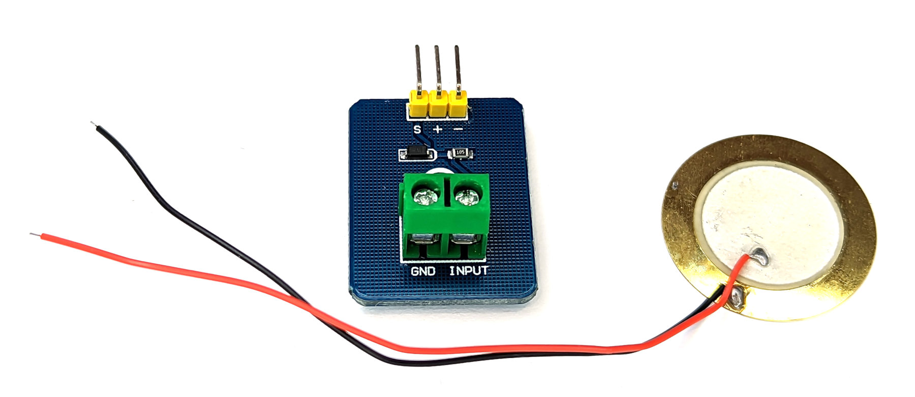
The interface board will connect to the Pico as an analogue device with the addition of a power supply connection that can be used at 5 or 3.3V.

Connecting everything up

We will want to connect;

• + on the interface board to the 3V3 pin (36) on the Pico
• - on the interface board to the Ground pin (38) on the Pico
• S on the interface board to ADC0 pin (31) on the Pico

The power and ground pins are fairly self explanatory, and because the vibration sensor’s interface board has an analogue output, we will apply signal output (S) to one of our Analogue to Digital Converter (ADC) pins. In this case ADC0 on pin 31 (GPIO26).

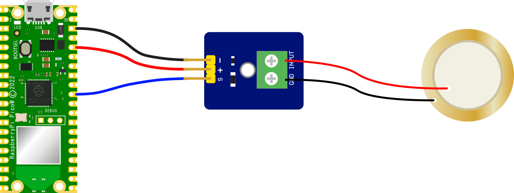
Connecting the interface board to the Pico practically can be achieved in a number of ways. But because the connection is relatively simple we can build a minimal configuration that will plug directly onto the pins using Dupont header connectors and jumper wire.

Code

The following code takes 20 readings from the analogue connection on GPIO26 (ADC0) in quick succession. It then discards the maximum and minimum values in the set and averages the remainder. This is done so that the sensor can get a ‘reading’ of a vibration that represents a value over a slightly longer period of time than a single reading. This is useful since the sensor can respond so quickly to a movement, that it may be possible for low frequency vibrations or impacts to not get a true representation

from machine import ADC, Pin
import time

# Sensor reading connection 
adc = ADC(Pin(26))

# Number of repetitions per reading
n = 20

while True:
    reading_group = []
    
    for x in range(n):
        new_value = adc.read_u16()
        reading_group.append(new_value)
        time.sleep(.01)
    
    # Get rid of the outliers
    reading_group.remove(max(reading_group))
    reading_group.remove(min(reading_group))
    
    # Get the average
    vibration = sum(reading_group)/ len(reading_group)
    
    print(vibration)

To test the code we can run it with the sensor taped to a suitably ‘vibrat-y’ device. I tried both a electric knife and a battery powered jig-saw. Both produced good results. Ultimately I have a plan in mind to attach them to my water pump to tell how long it is operating for and to the aeration pump on my septic system (that runs continuously) so that I can be alerted if it fails or if part of it fails (like a diaphragm) which would alter the nature of the vibration.

Using an Inertial Measurement Unit (IMU) with a Pico

This project will connect a 6 Degrees of Freedom (DoF) IMU to our Raspberry Pi Pico and demonstrate it’s use.

The IMU

An Inertial Measurement Unit, is a device that consists of one or more sensors that measure specific types of physical quantities, such as acceleration, angular velocity, and magnetic field strength. These sensors are typically arranged in a package that includes a microprocessor to process the sensor data and output the measured quantities in a usable form. IMUs are often used in applications that require precise measurements of motion, orientation, or position, such as in drones, robots, and virtual reality systems

IMUs have been around for several decades and have undergone significant development over time. Early IMUs were relatively simple devices that used mechanical sensors, such as gyroscopes and accelerometers, to measure motion and orientation. These sensors were often large and expensive, and the resulting IMUs were not very portable or practical for many applications.

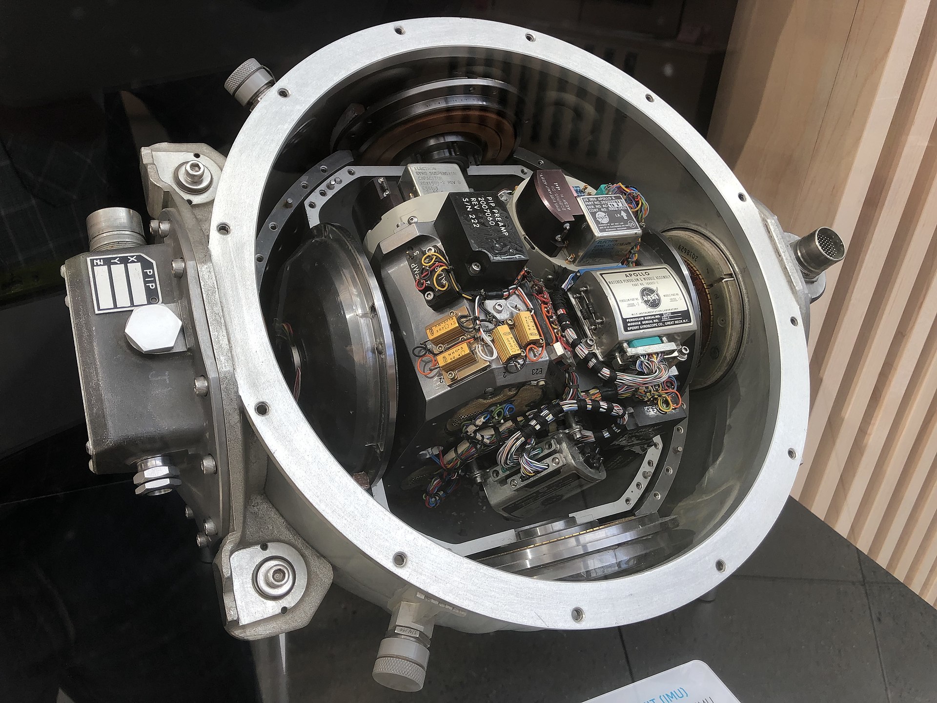
In the last few decades, there has been a shift towards using microelectromechanical systems (MEMS) sensors in IMUs. These sensors are much smaller and more affordable than their mechanical counterparts, and they have greatly increased the portability and accessibility of IMUs.

IMU’s are typically defined by the numbers of ‘Degrees of Freedom’ (DoF) they are capable of measuring.

• 6 DoF: Includes a three axis accelerometer and a three axis gyroscope.
• 9 DoF: Includes the elements of a 6 DoF unit and a three axis magnetometer.
• 10 DoF: Includes the elements of a 9 DoF unit and a barometer.

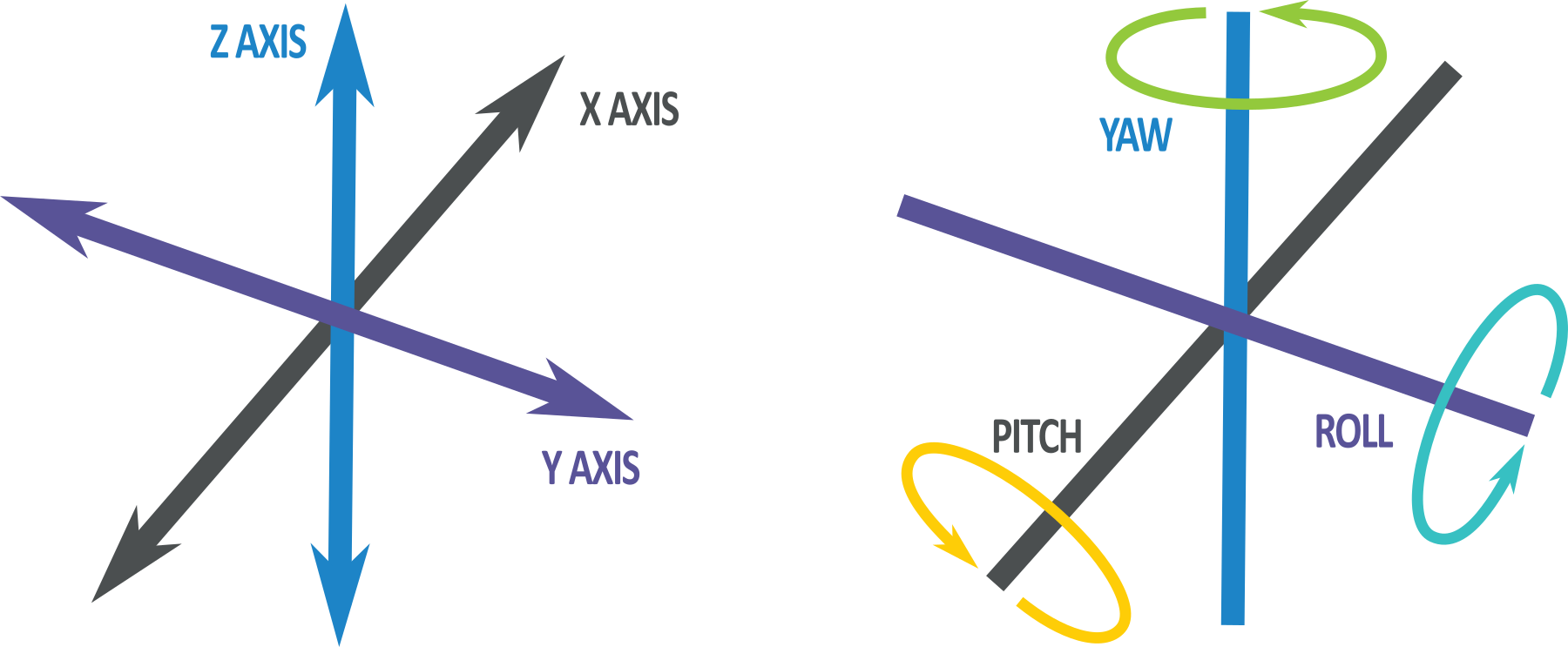
In addition to the sensors themselves, modern IMUs also typically include a microprocessor that is capable of processing the sensor data and outputting it in a usable form. This allows the IMU to provide real-time measurements of motion, orientation, and position, which can be used in a variety of applications.

The unit we will connect to is capable of measuring 6 degrees of freedom.

3-axis Accelerometer

A MEMS (Microelectromechanical Systems) 3-axis accelerometer is a small, lightweight device that measures acceleration along three orthogonal axes (typically labeled as x, y, and z). It can be used to detect the magnitude and direction of gravitational acceleration, as well as any additional acceleration that may be caused by movement or vibration.

Accelerometers are commonly used in a variety of applications and can be used to detect the orientation of the device relative to a reference frame, to measure the acceleration of the device during movement, or to detect and respond to impacts or other types of mechanical shock.

MEMS accelerometers typically use a small mechanical structure, such as a proof mass, that is suspended on a flexible beam or membrane. When the device is subjected to acceleration, the proof mass is displaced from its equilibrium position, and this displacement is detected by a sensor, such as a capacitive or piezoresistive transducer. The sensor output is then processed by an electronic circuit to determine the magnitude and direction of the acceleration.

MEMS accelerometers are often small and inexpensive, and they can operate over a wide temperature range. They are also relatively low power and have a fast response time, which makes them well-suited for use in portable and mobile applications.

3-axis Gyroscope

A MEMS (Microelectromechanical Systems) 3-axis gyroscope is a small, lightweight device that measures angular velocity along three orthogonal axes (typically labeled as x, y, and z). It can be used to detect the rate of rotation around these axes, and can be used to determine the orientation of the device relative to a reference frame.

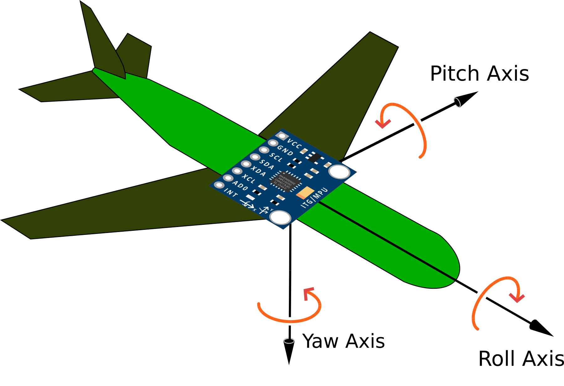
Gyroscopes are commonly used in a variety of applications that require precise measurement of motion or orientation, such as in drones, robots, and virtual reality systems. They can be used to stabilize the motion of a device, to navigate through unknown environments, or to track the orientation of the device over time.

MEMS gyroscopes typically use a small mechanical structure, such as a spinning rotor or a vibrating element, that is suspended on a flexible beam or membrane. When the device is subjected to angular velocity, the rotor or vibrating element responds by changing its position or motion, and this change is detected by a sensor, such as a capacitive or piezoresistive transducer. The sensor output is then processed by an electronic circuit to determine the magnitude and direction of the angular velocity.

MEMS gyroscopes are often small and inexpensive, and they can operate over a wide temperature range. They are also relatively low power and have a fast response time, which makes them well-suited for use in portable and mobile applications. However, they are subject to drift over time, which can limit their accuracy in certain applications.

The GY-521 IMU module using a MPU-6050

The GY-521 module is a breakout board for the MPU-6050. This is a 6-axis IMU that includes a 3-axis accelerometer and a 3-axis gyroscope. It is produced by InvenSense and is commonly used in a variety of applications that require precise measurements of motion, orientation, or position.

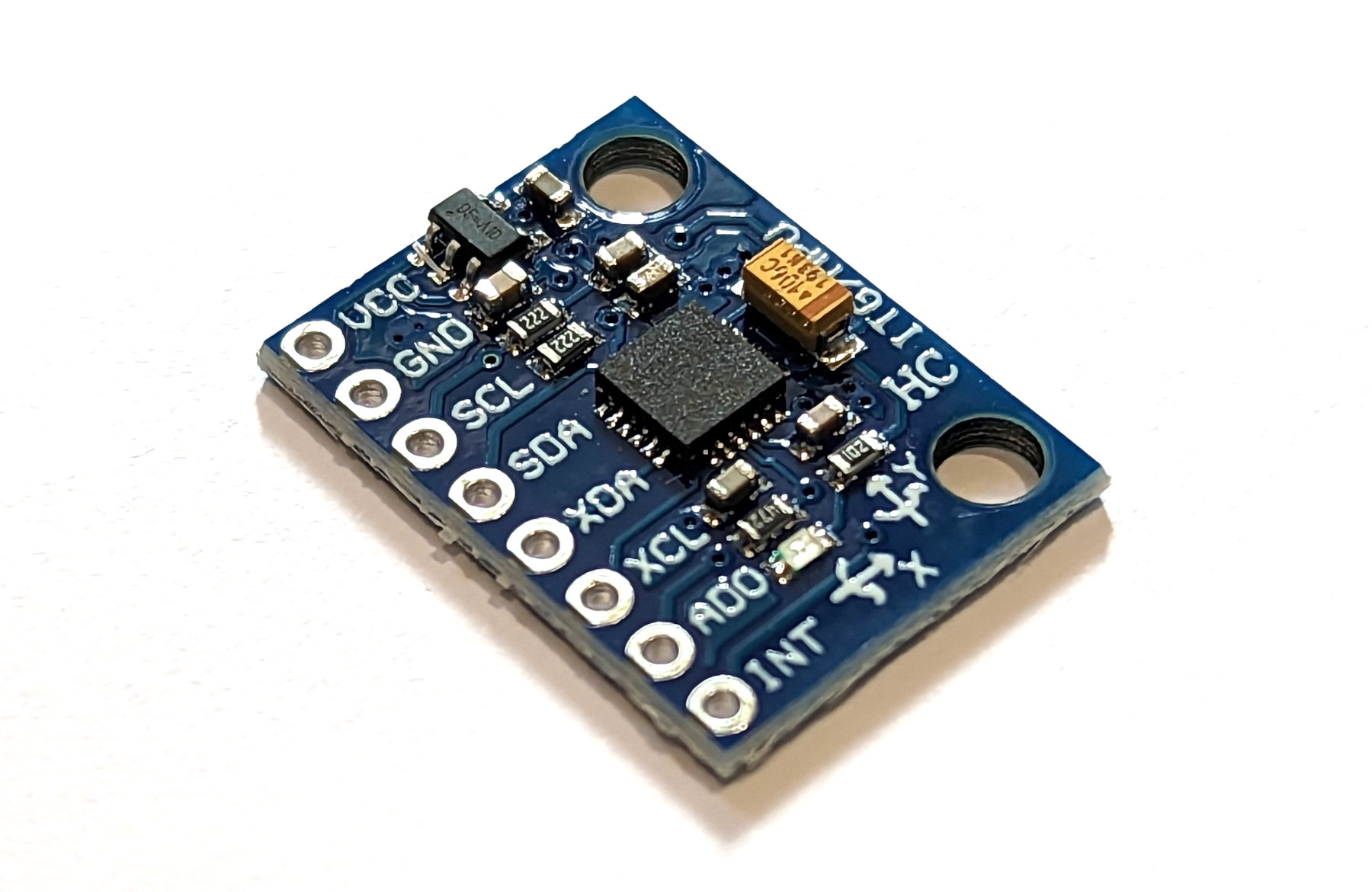
The accelerometer component of the MPU-6050 measures linear acceleration in the x, y, and z axes. It can be used to detect the magnitude and direction of gravitational acceleration, as well as any additional acceleration that may be caused by movement or vibration. The accelerometer measures the rate of change of velocity over time. It is sensitive to changes in motion and can be used to detect the direction and magnitude of acceleration, as well as changes in orientation.

The gyroscope component of the MPU-6050 measures angular velocity in the x, y, and z axes. It can be used to detect the rate of rotation around these axes, and can be used to determine the orientation of the device relative to a reference frame. The gyroscope measures angular velocity, which is the rate of change of orientation over time. It is sensitive to changes in rotational motion and can be used to detect the direction and magnitude of rotation, as well as changes in orientation.

The MPU-6050 also includes a built-in temperature sensor and a digital motion processor (DMP) that can be used to process the sensor data and output it in a usable form. The MPU-6050 communicates using an I2C or SPI interface, and it can be configured and controlled using register settings.

Connecting the GY-521 to the Raspberry Pi Pico

The connection is fairly simple with only four connecting wires being required. Power, ground, Serial CLock line (SCL) and Serial DAta line (SDA). The following connections are used for this example

• Connect the GY-521’s SDA (data) pin to the Pico’s I2C1 SDA (pin 31, or GPIO26) on the Pico (Brown).
• Connect the GY-521’s SCL (clock) pin to the Pico’s I2C1 SCL (pin 32, or GPIO27) on the Pico (Orange).
• Connect the GY-521’s VCC (power) pin to the Pico’s 3V3(OUT) (pin 36) power pin.
• Connect the GY-521’s GND (ground) pin to the Pico’s GND (pin 38) pin.

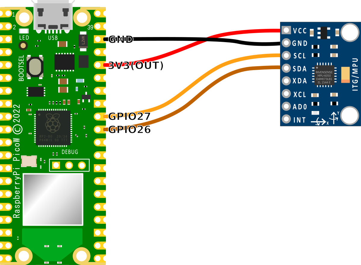
An important point to note when we are connecting our Pico is that because the RP2040 microcontroller has two I2C controllers, we need to ensure that we define which controller we are using in the code. I2C0 = id 0 and I2C1 = id 1. This is set in the following lines in the MicroPython code;

i2c = I2C(1, sda=Pin(26), scl=Pin(27), freq=400000)

In our case, since we are using GPIO26 and GPIO27 for the SDA and SCK connections we are using I2C Controller 1.

Code

The values from the IMU are accessed via two pre-built MicroPython modules (imu.py and vector3d.py). These have been published on GitHub. To make use of the module we will need to download them from GitHub and then copy them over to our Pico. I found this most easily accomplished by first downloading the files to the main computer and then going File >> Open on Thonny and selecting the appropriate file. From there go File >> Save as… and select the Pico as the location to save the file (making sure to save it with the appropriate name).

The printed values from the code below represent the accelerometer and gyroscope readings of the MPU-6050 IMU in 3-dimensional space.

In this code, the x, y, and z values represent the readings in the respective axes. Positive values indicate that the IMU is accelerating or rotating in the positive direction of the respective axis, while negative values indicate that it is accelerating or rotating in the negative direction.

import time
from machine import I2C, Pin
from imu import MPU6050

# Set up I2C communication with the MPU-6050
i2c = I2C(1, sda=Pin(26), scl=Pin(27), freq=400000)

# Create an MPU6050 object with the I2C interface
imu = MPU6050(i2c)

# Set the full-scale range of the accelerometer (in g)
imu.accel.full_scale_range = 2

# Set the update rate of the loop (in Hz)
UPDATE_RATE = 10

# Main loop
while True:
    # Read the accelerometer and gyroscope values
    accel = imu.accel
    gyro = imu.gyro

    # Print the values to the terminal
    print("Acceleration x: {:+5.2f} y: {:+5.2f} z: {:+5.2f}    gyroscope x: {:+7.\
2f} y: {:+7.2f} z: {:+7.2f}".format(
        accel.x, accel.y, accel.z, gyro.x, gyro.y, gyro.z), end='\r')

    # Wait a moment before reading again
    time.sleep(1.0 / UPDATE_RATE)

The time and machine modules are imported, along with the MPU6050 class from the imu module.

The I2C interface is set up using the I2C class from the machine module, with the sda and scl pins connected to pins 26 and 27 on the Raspberry Pi, respectively. The frequency of the I2C bus is set to 400000 Hz.

An MPU6050 object is created with the I2C interface. This object will be used to communicate with the IMU and read the accelerometer and gyroscope values.

The full-scale range of the accelerometer is set to 2 g. This determines the maximum range of the accelerometer readings, with higher values corresponding to a larger range.

The main loop begins and the accelerometer and gyroscope values are read using the accel and gyro properties of the MPU6050 object. These properties are objects that contain the x, y, and z components of the acceleration and angular velocity vectors, respectively.

The print section outputs the values to the terminal in a format that makes it easy to read (but not necessairly easy to write!)

Using an OLED Display attached to a Pico

This project will use an attached OLED display unit to present information from our Raspberry Pi Pico.

The OLED Display

The display that we’ll use in this example is based on the SSD1306 driver chip, which acts as a bridge between the display matrix and the Pico. The matrix can come in a variety of resolutions (128x64, 128x32, 72x40, 64x48) and colours (white, yellow, blue). The display itself uses an organic light-emitting diode (OLED) technology that allows it to be bright, fairly detailed and to have a wide viewing angle. It also doesn’t hurt that the device is also very reasonably priced.

The specifications of the unit used here is 0.96 inches on the diagonal, has a resolution of 128x64 and is white on a black background.

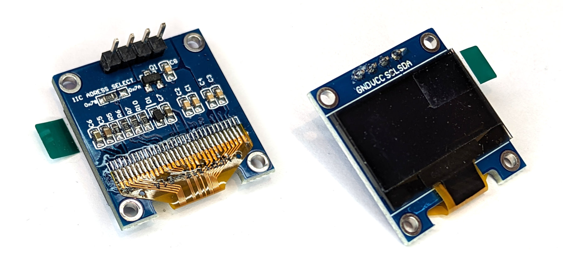
The green tab on the side is simply there to make removal of the protective film on the screen easy.

The SSD1306 micro-chip driver uses an I2C communications protocol and there is a PyPI library available that can be used for basic controls. There are some models that will also include SPI connectivity and these can be identified by having more than the four connecting pins that are shown on the model above. For more information on the unit we can consult the datasheet.

Connecting the Display to the Pico

The connection is fairly simple with only four connecting wires being required. Power, ground, Serial CLock line (SCL) and Serial DAta line (SDA). The following connections are used for this example;

• Display GND to Ground (pin 38) on the Pico (Black)
• Display VIN to the 3V3(OUT) (pin 36) on the Pico (Red)
• Display SCL to I2C1 SCL (pin 32, or GPIO27) on the Pico (Orange)
• Display SDA to I2C1 SDA (pin 31, or GPIO26) on the Pico (Brown)

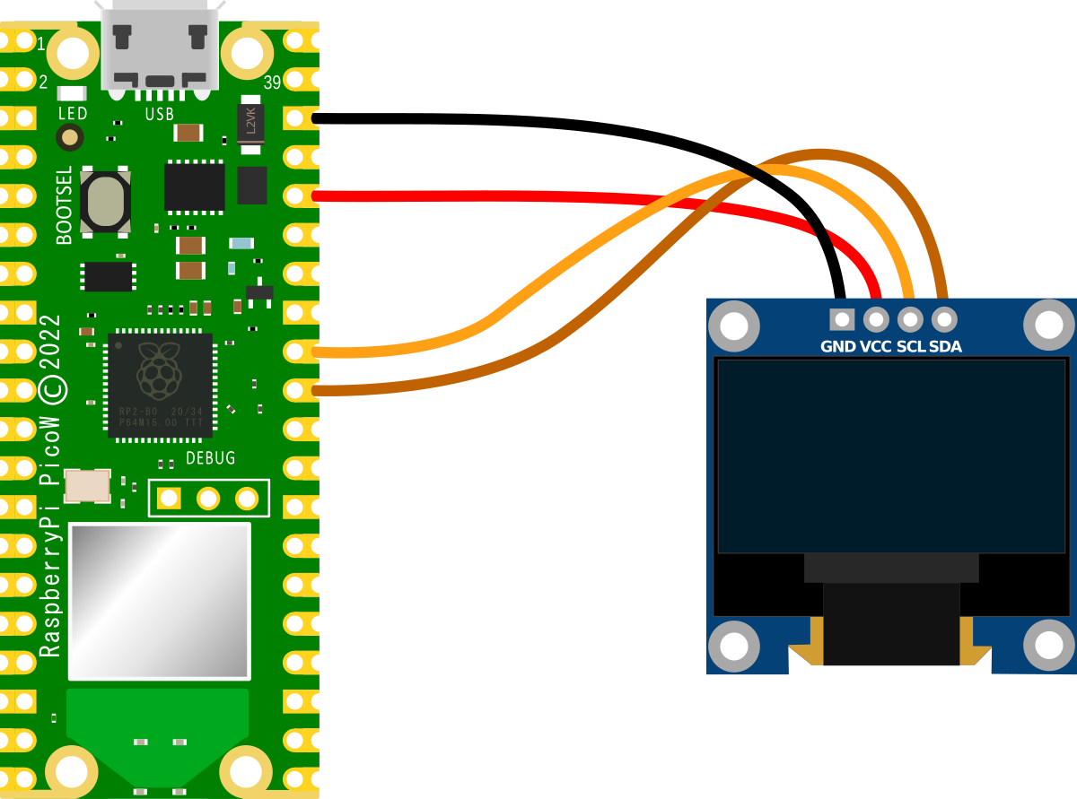
An important point to note when we are connecting our Pico is that because the RP2040 microcontroller has two I2C controllers, we need to ensure that we define which controller we are using in the code. I2C0 = id 0 and I2C1 = id 1. This is set in the following lines in the MicroPython code;

i2c = I2C(1, sda=sda, scl=scl)

In our case, since we are using GPIO26 and GPIO27 for the SDA and SCK connections we are using I2C Controller 1.

Loading the ssd1306 PyPI module

The display is accessed via I2C, but we can abstract the complexities of this via a pre-built MicroPython library. To make use of the library we will use Thonny to find and download it.

1. With our Pico connected to our desktop computer, open Thonny.
2. Click on Tools > Manage Packages to access Thonny’s package manager.
3. Type ‘ssd1306’ in the search bar and click on ‘Search on PyPI’. This will return a few results.
4. Click on ‘micropython-ssd1306’ (ssd1306 module for MicroPython) and then click on ‘Install’. This will copy the library to our Pico.

Click on ‘Close’ to return to the main screen.

And that’s it, we’re all set up to use the ‘ssd1306’ library.

Code

The code below is incredibly basic and aimed at providing an example of how easy it it is to get started using the display. There is a great deal more that can be done with the display to add shapes, pictures and movement, but our aim is to get up and running and then from there we can push on to greater things :-).

The code below will print ‘Pico’ five times staggered across the screen.

from machine import Pin, I2C
from ssd1306 import SSD1306_I2C

# Create I2C object
sda = Pin(26)
scl = Pin(27)
i2c = I2C(1, scl=scl, sda=sda, freq=400000)

oled = SSD1306_I2C(128, 64, i2c)

oled.text("Pico", 0, 0)
oled.text("Pico", 20, 10)
oled.text("Pico", 40, 20)
oled.text("Pico", 60, 30)
oled.text("Pico", 80, 40)

oled.show()

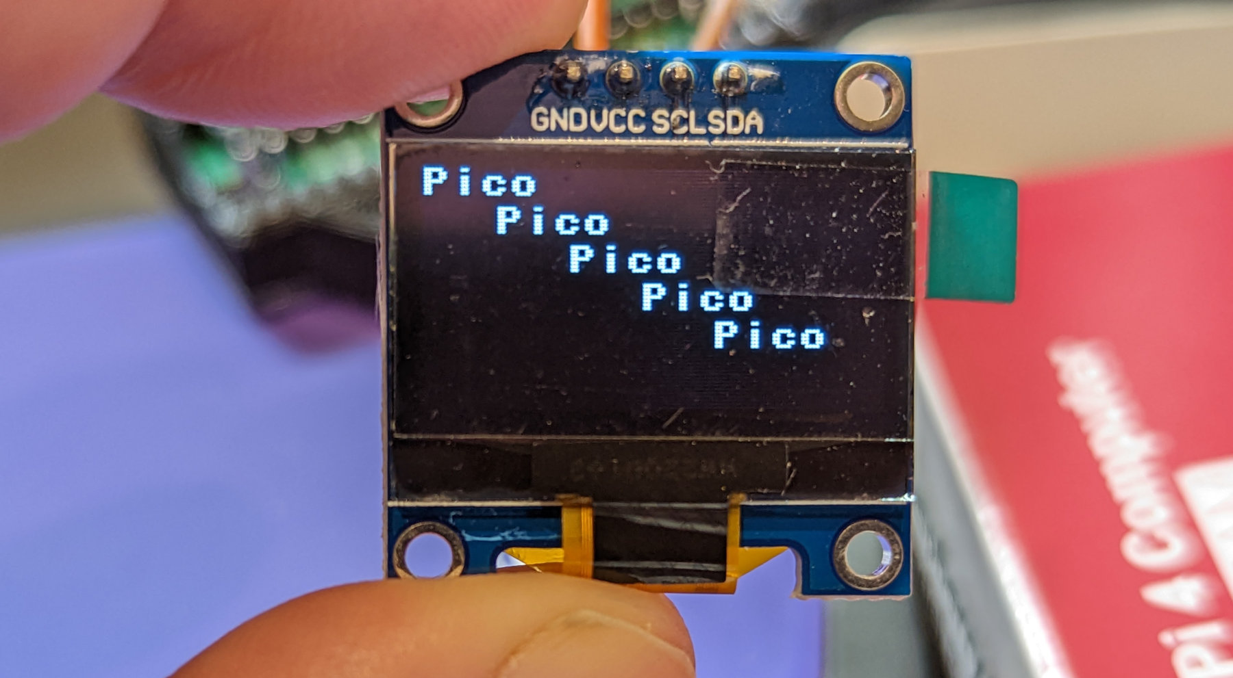
While the example above is limited, we can also use some of the code’s functions available for the display to add greater complexity. Feel free to have a play with some of the options below;

oled.poweroff()     # power off the display, pixels persist in memory
oled.poweron()      # power on the display, pixels redrawn
oled.contrast(0)    # dim
oled.contrast(255)  # bright
oled.invert(1)      # display inverted
oled.invert(0)      # display normal
oled.rotate(True)   # rotate 180 degrees
oled.rotate(False)  # rotate 0 degrees
oled.show()         # write the contents of the FrameBuffer to display memory

For greater illustration of what can presented on the display, check out the MicroPython docs page for the ESP8266 which presents further options.

And as a final tribute to the MicroPython instructions, run the following code;

from machine import Pin, I2C
from ssd1306 import SSD1306_I2C

# Create I2C object
sda = Pin(26)
scl = Pin(27)
i2c = I2C(1, scl=scl, sda=sda, freq=400000)

oled = SSD1306_I2C(128, 64, i2c)

oled.fill(0)
oled.fill_rect(0, 0, 32, 32, 1)
oled.fill_rect(2, 2, 28, 28, 0)
oled.vline(9, 8, 22, 1)
oled.vline(16, 2, 22, 1)
oled.vline(23, 8, 22, 1)
oled.fill_rect(26, 24, 2, 4, 1)
oled.text('MicroPython', 40, 0, 1)
oled.text('SSD1306', 40, 12, 1)
oled.text('OLED 128x64', 40, 24, 1)

oled.show()

Enjoy!

Using a Dot-Matrix Display Attached to a Pico

A dot matrix display is a little like a compromise between the simplicity of a seven segment display and a modern screen. They have a lot of flexibility and through widely available Python modules can be easily used with a Raspberry Pi Pico.

The Dot-Matrix Display

The display is an array of LEDs that can be lit in patterns to represent text, patterns and images. This tutorial will use the MAX7219 dot matrix display to demonstrate how easily they can be used. There is a good chance that you may have seen a MAX7219 module at some point since they are relatively common and inexpensive and therefore popular as a solution for display based projects. They have the additional advantage of being able to be connected together to create larger arrays and therefore images.

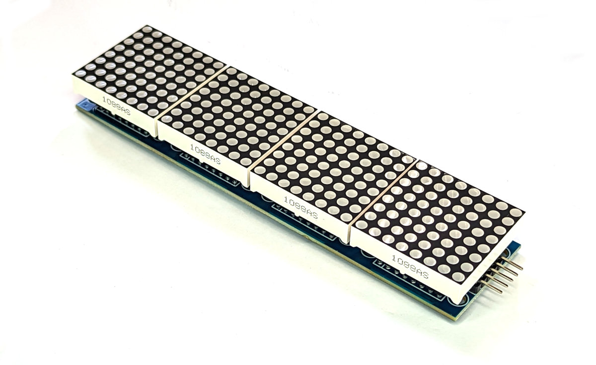
How is the display accessed?

The display is accessed via SPI, but we can abstract the complexities of this via a pre-built MicroPython module. This has been published on GitHub by FideliusFalcon. To make use of the module we will need to download it from GitHub and then copy it over to our Pico. I found this most easily accomplished by first downloading the file to the main computer and then going File >> Open on Thonny and selecting the appropriate file. From there go File >> Save as… and select the Pico as the location to save the file (making sure to save it with the appropriate name (max7219.py)).

Because of the abstraction afforded by the library, the reading of the sensor is nicely simplified.

Connecting the Display to the Pico

While under normal conditions SPI interfaces rely on sending and receiving data, in this application the Pico only sends. Therefore, while we would normally include a MISO (master in, slave out) connection on the peripheral, in this case it is not required. As always, since there are a range of different ways for labelling SPI-compatible signalling lines, try not to second guess things and figure it out, The connection diagram below is correct. The table below also makes an attempt to match up the naming conventions, but honestly, the diagram is our best benchmark.

Function                SPI   Pico      MAX7219
Output from controller  MOSI  SPI0 TX   DIN
Input to controller     MISO  SPI0 RX   N/A
Clock                   SCK   SPI0 SCK  CLK
Chip select             CS    SPI0 CSN  CS

The display module is labelled ‘DIN’, ‘SCK’ and ‘CS’, so the wiring should be relatively clear (but look to the connection diagram if in doubt). As with so many of these connections, some simple Dupont connecting wires will suffice.

Code

The code below rotates the words ‘RPi’ and ‘Pico’ on the display. Take the opportunity add your own text and adjust the brightness settings to get a feel for the variations that are possible.

from machine import Pin, SPI
import max7219
from time import sleep

spi = SPI(0,sck=Pin(18),mosi=Pin(19))
cs = Pin(17, Pin.OUT)

display = max7219.Matrix8x8(spi, cs, 4)

display.brightness(10)

while True:

    display.fill(0)
    display.text('RPi',0,0,1)
    display.show()
    sleep(3)
    
    display.fill(0)
    display.text('PICO',0,0,1)
    display.show()
    sleep(3)

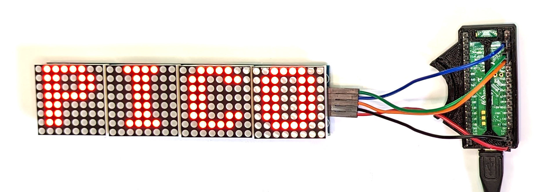
Scrolling

Showing text is one thing, but scrolling text is another :-). The code below takes a string of text and moves it across the face of the display.

from machine import Pin, SPI
import max7219
import time

#Intialize the SPI
spi = SPI(0, baudrate=10000000, polarity=1, phase=0, sck=Pin(18), mosi=Pin(19))
cs = Pin(17, Pin.OUT)

display = max7219.Matrix8x8(spi, cs, 4)

display.brightness(0)
scrolling_message = "RASPBERRY PI PICO SCROLLING DISPLAY"
length = len(scrolling_message)

column = (length * 8)

display.fill(0)
display.show()

time.sleep(1)

while True:
    for x in range(32, -column, -1):     
        display.fill(0)
        display.text(scrolling_message ,x,0,1)
        display.show()
        time.sleep(0.05)

In this instance, play with the message and the sleep time to adjust what is being displayed and the speed of movement.

Controlling addressable LEDs

The Raspberry Pi Pico can be used to provide lighting control to create effects and custom illumination via individually addressable LEDs that can be combined in a range of configurations. The applications could range from a simple colour changing accent light to a wearable display to a light sabre.

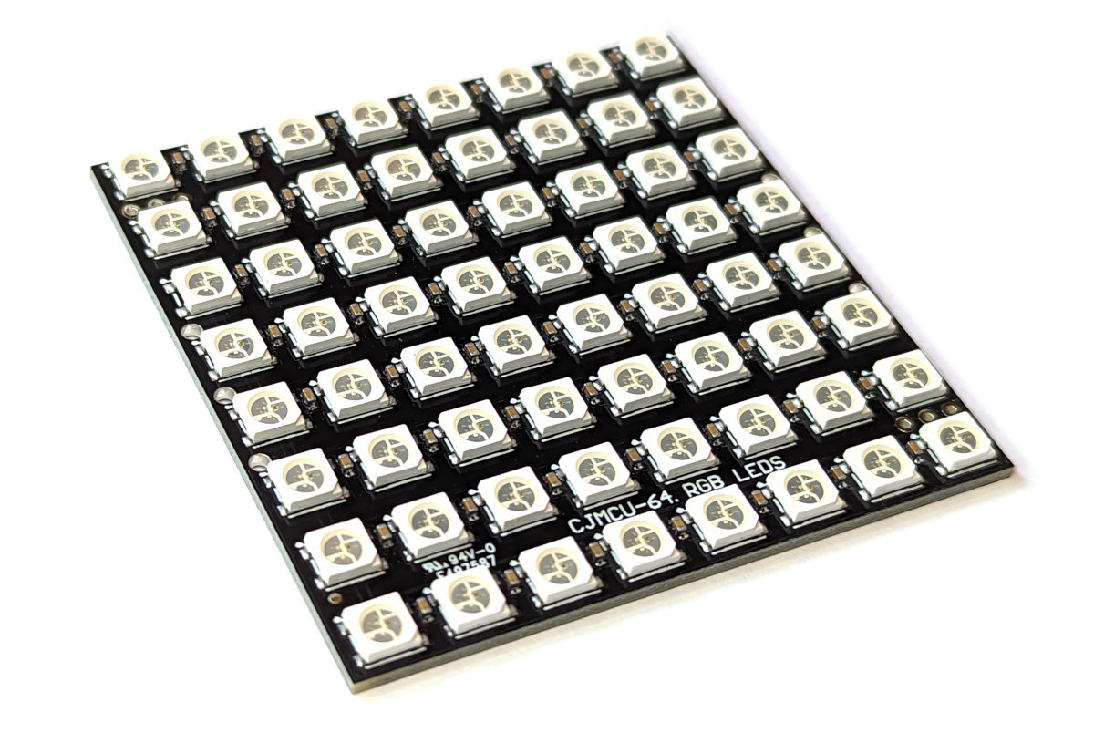
What are addressable LEDs?

Addressable LEDs are lights that have unique controllers built in that allow us to adjust the properties of individual LEDs or groups of them ganged together in strips, matrices or other patterns. The ability to control a specific LED is why they are referred to as ‘addressable’. Having this function available allows us to create different effects for a single LED either on its own or as part of a larger display.

There are a variety of configurations for addressable LEDs. As well as the different pattern configurations (strips, matrices etc.) they can come in different densities, colour, weather proofing, and connectivity options.

The most significant feature of addressable LEDs is the type of integrated controller chip that they use. The three most common are;

• WS2811
• WS2812B
• WS2813

WS2811

The WS2811 is normally found in 12V installations. 12V is preferable if we want to connect up longer lengths of LEDs to reduce the effects of voltage drop with distance. This aids in providing better colour consistency.

As we are going to be using the Pico, the added complexity of using a different voltage source for the LEDs and the Pico is not going to be an advantage.

One of the most popular brands of addressable LEDs are made and distributed by Adafruit and are called NeoPixels. They have put a lot of effort into developing and supporting this product and I thoroughly recommend that you take a look.

WS2812B and WS2813

There is an older version of the WS2812B called the WS2812. The older version utilised a six pin connection which made connection slightly more complicated, and the newer version improved the mechanical properties of the package along with better heat dissipation, higher brightness and reverse power protection.

The WS2812B is a less advanced option than the WS2813. While both will typically operate from a 5V source, the WS2813 has a higher refresh rate (2000Hz vs 400Hz) and it includes a backup signalling channel which will make larger arrays of the LEDs more tolerant to individual failure.

The recommended power injection interval on the WS2812B is higher (5m vs 2.5m for the WS2813) which makes longer runs when configured in strips easier.

How do addressable LEDs work?

Each addressable LED includes the LED proper (typically a 5050 RGB model) which is a combination of three separate Red, Green and Blue (RGB) LEDs in a 5mm x 5mm package with a controller IC (the aforementioned WS2812B or WS2813).

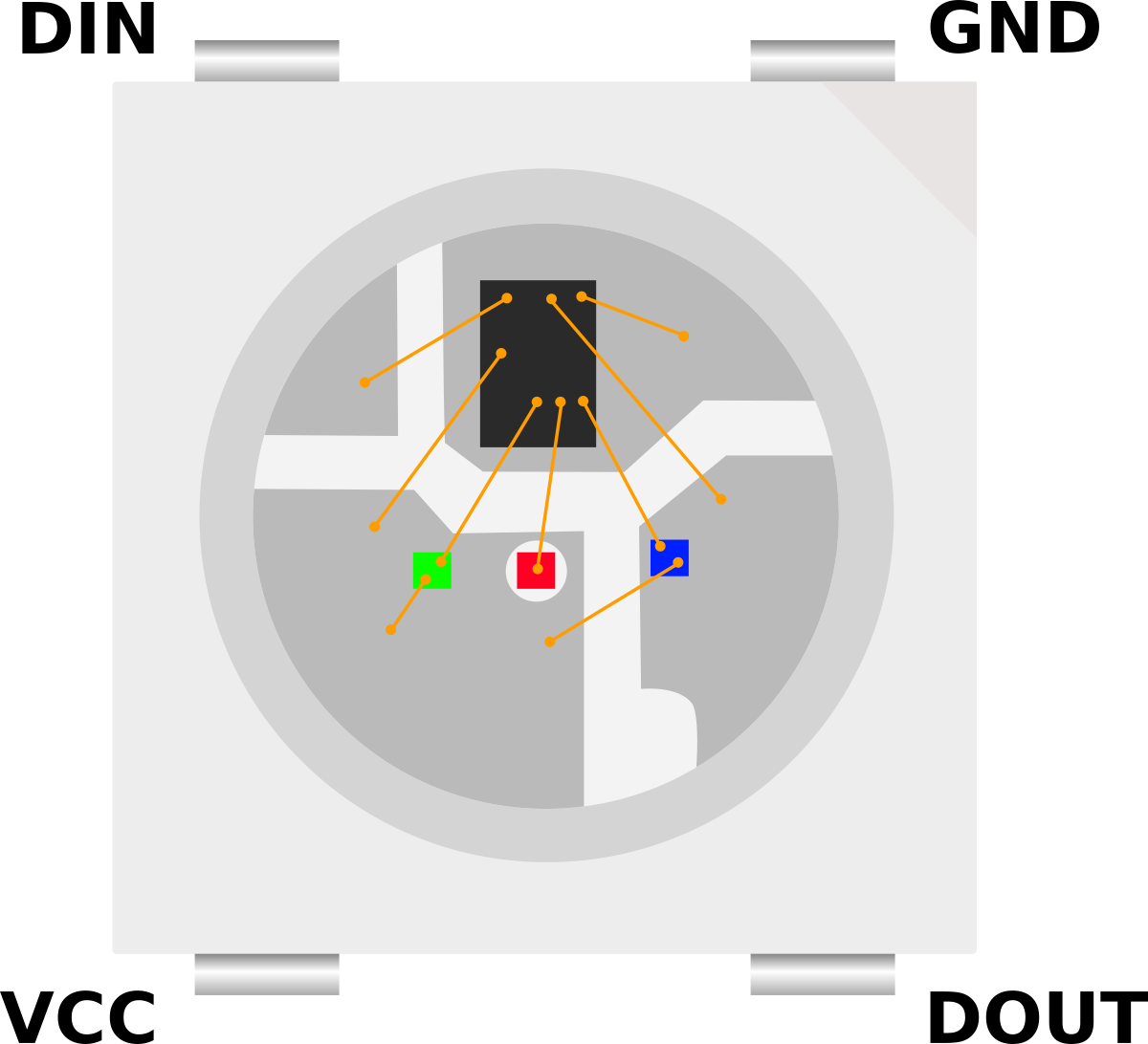
Each package has four pins – VCC, Ground, DIN (Data IN), and DOUT (Data OUT). The controlling connection from our Pico goes to the DIN pin and follow on LEDs are daisy chained from the initial devices DOUT pin to the follow on devices DIN. Thus, the controlling signal only requires a single wire from our Pico (Although it will still require power in the form of VCC (5V) and ground).

Each separate red, green, and blue LED in the package can be set to shine at one of 256 brightness levels. The combination of those three colours at different levels of brightness allows for the generation of the full colour spectrum. The signal sent from our Pico will be a sequence of RGB combinations which will go to the first connected LED. This receives the first set of RGB levels and passes the remainder through to the follow on LED. This in turn receives the next set of levels and passes on the remainder etc, etc, until the end of the line (signals or LEDs) is met.

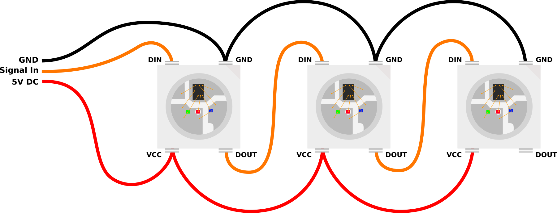
Signal Voltage Level

While we have discovered above that there are 12V and 5V versions of the LEDs that can be used for these applications, the 5V versions are the most prevalent. However, if we look at the datasheets for the devices (WS2812 WS2812B, WS2813) we can see that they generally have a fairly loose range of supply voltages (VCC) that will power them, but the voltages for the signal line on DIN are a proportion of the supply voltage. A signal ‘high’ is 0.7 x VCC and a ‘low’ is 0.3 x VCC.

Meaning that if we were supplying exactly 5V to power one of the LEDs, we would require a voltage of 3.5V for the LED to recognise the signal as a logical ‘high’. “Hang on” I hear you say. “Our Raspberry Pi Pico will only send out a 3.3V signal as a ‘high’ when it is connected to a GPIO pin”. Yep. Well spotted. So what’s that all about?

Well… The required signal levels in these cases are a little like the pirate’s code. It turns out that they are more of a ‘guideline’ than a hard and fast rule.

I have yet to come across an addressable LED device that didn’t work with 3.3V signalling if VCC is set at 5V. That’s not to say that it won’t happen, but at the time of writing, that has been my experience.

If we wanted to make sure that we were being faithful to the requirements of the datasheet we could employ the services of a ‘level shifter’ or ‘logic level converter’ that will change our logic levels from one voltage to another.

Power Requirements

Each individual LED can draw up to 60mA of current. That’s not a huge amount in the scheme of things, but because addressable LEDs are typically packaged as strips or matrices, if we multiply that current draw by the possible number of LEDs in a connection, the value starts to be come significant.

For instance, a 1m strip with 30 LED’s could potentially draw up to 1.8A of current. That’s quite a lot and to be honest, it’s a worst case scenario. For general use where we would be varying our colours and brightness to make pretty patterns, we can probably work on a rule of thumb that 20mA per LED is about right.

Our Pico has a direct connection from the USB connector to the VBUS connector (where we are taking our 5V supply from for our LEDs) so that means that we are dependant on our power supply to our Pico in terms of managing the appropriate amount of power if we are feeding our LEDs from the Pico.

If we were using a larger number of connected LEDs it might be necessary to divide your strip into different sections and connect separate power supplies. This could be because you need a certain amount of current to drive the LEDs or it could be because of the voltage drop that will occur over longer distances due to the resistance of the copper connecting wires.

Important points to note when doing this is that the ground wires are all connected together and the signal chain is contiguous, but the positive power line is separated into its different sections.

Connecting the addressable LEDs

As described above, the connection will depend a little on what LED module you are using and whether or not you determine that you might need a logic level converter, but for 95% (I’m speculating wildly with this figure BTW) of connections you should be able to simply connect as follows;

         Pico    LEDs
Voltage  VBUS    +5V
Ground   GND     GND
Signal   GPIOxx  DIN

Keeping in mind that we are utilising the GPIO26 pin in this example for simplicity’s sake. You should be able to use any GPIO pin. You will need to adjust the pin number in the code samples below however.

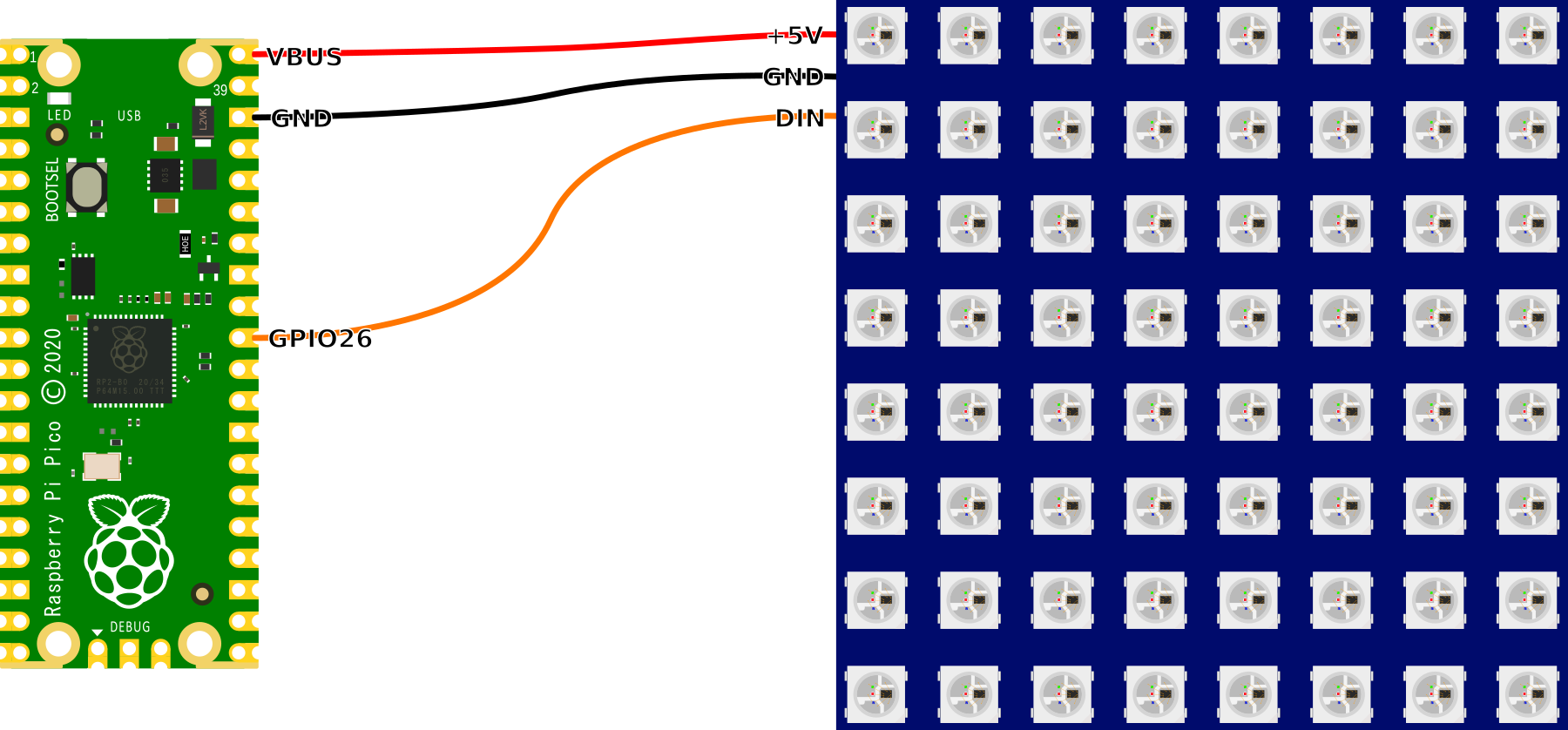
How do we talk to our addressable LEDs?

The LEDs are accessed via a pre-built MicroPython module. This has been published on GitHub by Blaž Rolih. To make use of the module we will need to download it from GitHub and then copy it over to our Pico. I found this most easily accomplished by first downloading the file to the main computer and then going File >> Open on Thonny and selecting the appropriate file. From there go File >> Save as… and select the Pico as the location to save the file (making sure to save it with the appropriate name (neopixel.py)).

Code

Scroll a red LED through all the pixels

from utime import sleep
# We are using https://github.com/blaz-r/pi_pico_neopixel
from neopixel import Neopixel

NUMBER_PIXELS = 64
STATE_MACHINE = 0
LED_PIN = 26

strip = Neopixel(NUMBER_PIXELS, STATE_MACHINE, LED_PIN, "GRB")

# Color RGB values
red = (255, 0, 0)
off = (0,0,0)

delay = .1
while True:
    for i in range(0, NUMBER_PIXELS):
        strip.set_pixel(i, red)
        if i > 0: strip.set_pixel(i-1, off)
        if i == 0: strip.set_pixel(NUMBER_PIXELS-1, off)
        strip.show()
        sleep(delay)

This code (led-red-run.py) is available to download (at no cost) as an extra from Leanpub when you download the book

Run two LEDs around the outside of a 8 x 8 matrix.

from utime import sleep
# We are using https://github.com/blaz-r/pi_pico_neopixel
from neopixel import Neopixel

NUMBER_PIXELS = 64
STATE_MACHINE = 0
LED_PIN = 26

strip = Neopixel(NUMBER_PIXELS, STATE_MACHINE, LED_PIN, "GRB")

# Color RGB values
red = (255, 0, 0)
off = (0,0,0)

delay = .1
while True:
    for i in range(0, 8):
        strip.set_pixel(i, red)
        if i > 0: strip.set_pixel(i-1, off)
        if i == 0: strip.set_pixel(63, off)
        strip.set_pixel(i*8, red)
        if i > 0: strip.set_pixel((i-1)*8, off)
        strip.show()
        sleep(delay)
    for i in range(1, 8):
        strip.set_pixel(56+i, red)
        if i > 1: strip.set_pixel(56+(i-1), off)
        if i == 1: strip.set_pixel(56, off)
        strip.set_pixel(((i+1)*8)-1, red)
        strip.set_pixel(((i)*8)-1, off)
        #if i > 1: strip.set_pixel(((i-1)*8)+7, off)
        strip.show()

This code (led-8x8-outside.py) is available to download (for free) as an extra from Leanpub when you download the book

There are a couple more code samples available for download from Leanpub.

• led-8x8-squares.py which cycles squares in and out of an 8x8 matrix.
• led-8x8-squares.py which cycles lines to and fro on a 8x8 matrix.
• led-random.py which flashes random colours on random pixels in a matrix or a strip (just set the number of pixels).

Using the Raspberry Pi Pico as a Prometheus Node

About Prometheus and Grafana

Prometheus is an open source application used for monitoring and alerting. It records real-time metrics in a time series database built using a HTTP ‘pull’ model.

It was was created because of the need to monitor multiple microservices that might be running in a system. It employs a modular architecture and employs modules called exporters, which allow the capture of metrics from a range of platforms, IT hardware and software.

Prometheus’s ‘pull model’ of metrics gathering means that it will actively request information for recording. It collects metrics at regular intervals and stores them locally. These metrics are pulled from nodes that run ‘exporters’. An exporter can be defined as a module that extracts information and translates it into the Prometheus format.

Prometheus data is stored as metrics, with each having a name that is used for referencing and querying. This is what makes it very good at recording time series data.

Prometheus is commonly used in combination with the Grafana platform which has a very powerful visualisation capability.

I have written a separate book on installing and using Prometheus and Grafana here and I would recommend it to anyone who is interested in monitoring their physical or IT environment.

Using the Pico as an Exporter

This particular guide will describe how to use the Raspberry Pi Pico W as an exporter node. This will allow the distribution of simple sensors to be even more widespread than is possible with a Raspberry Pi Zero or similar since they are cheaper and have lower power requirements.

There isn’t a dedicated Prometheus exporter available for the Pico, so we will make one ourselves.

The good news is that when gathering metrics for use in a Prometheus / Grafana stack installation, metrics can be made available from a device via a simple web query that details various metric values for consumption.

The information presented on the web page is set out in the exposition format published here.

In its most simple form the information can take the format of a metric name and a value separated by any number of blank spaces or tabs. If more than one line (metric) is being presented, these must be separated by a line feed character (\n). The last line must end with a line feed character. Empty lines are ignored.

For example;

weather_inside_temperature_C 21.7
weather_barometer_mb 1035.6
weather_sunshine_hours_hours 11.0

A great deal more complexity can be integrated into the metric values including label names, and a time-stamp, but for the purposes of demonstrating the technique we will focus on a very simple example. For guidance on best practices for naming conventions and metric formatting in general, see the page on writing exporters here.

It is worth reinforcing here that this code is dependant on using the Pico W since it provides the mechanism for connecting to the Prometheus platform via a web request.

Code

The astute reader will recognise the following as being heavily based on the example used earlier in the book to serve a web page from the Pico W. Well spotted. You can also download this code as an extra with the book. It is bundled with the code samples extra and is called prometheus.py.

import network
import socket
import time
import random
import rp2

from secrets import secrets

ssid = secrets['ssid']
password = secrets['pw']

# Set country to avoid possible errors
rp2.country('NZ')

wlan = network.WLAN(network.STA_IF)
wlan.active(True)
wlan.connect(ssid, password)
wlan.ifconfig(('10.1.1.161','255.255.255.0','10.1.1.1','8.8.8.8'))

html = """# HELP pico_temp Temperature in C
# TYPE pico_temp gauge
pico_temp pico_temperature
# HELP pico_rand An Indication of a random number
# TYPE pico_rand gauge
pico_rand pico_random
"""

# Wait for connect or fail
max_wait = 10
while max_wait > 0:
    if wlan.status() < 0 or wlan.status() >= 3:
        break
    max_wait -= 1
    print('waiting for connection...')
    time.sleep(1)

# Handle connection error
if wlan.status() != 3:
    raise RuntimeError('network connection failed')
else:
    print('connected')
    status = wlan.ifconfig()
    print( 'ip = ' + status[0] )

# Open socket
addr = socket.getaddrinfo('0.0.0.0', 80)[0][-1]
s = socket.socket()
s.setsockopt(socket.SOL_SOCKET, socket.SO_REUSEADDR, 1)
s.bind(addr)
s.listen(1)
s.settimeout(120)
print('listening on', addr)

# Configure for reading temperature 
sensor = machine.ADC(4)

def temperature_reading():
    reading = sensor.read_u16()
    voltage = reading * ( 3.3 / 65535) 
    temperature = 27 - (voltage - 0.706) / 0.001721
    return(temperature)

# Listen for connections
while True:
    try:
        cl, addr = s.accept()
        print('client connected from', addr)

        request = cl.recv(1024)
        print(request)

        temperature = temperature_reading()
        rando = random.randint(0,99)

        print(rando)
        print(temperature)

        first = html.replace("pico_random",str(rando))
        last = first.replace("pico_temperature",str(temperature))
        
        response = last
        cl.send('HTTP/1.0 200 OK\r\nContent-type: text/html\r\n\r\n')
        cl.send(response)
        cl.close()

    except OSError as e:
        print('machine resetting')
        machine.reset()

This code combines several different components. It connects the Pico to a local network via WiFi. It sets itself a static IP address. It makes content available via port 80 so that it can be read by a browser. It serves content in an OpenMetric and Prometheus exposition format so that it can be read by Prometheus.

One of the more important parts of that is the setting of the static IP address via the following line;

wlan.ifconfig(('10.1.1.161','255.255.255.0','10.1.1.1','8.8.8.8'))

This is important so that we can tell Prometheus where to go to read the metrics. It’s important to remember from the section earlier in the book that these settings need to be particular to your network.

There is also a significant piece of code that differs from examples that a discerning reader might find on the interweb. Specifically the line;

s.settimeout(120)

We make this call when we are establishing our socket connection and it provides a countdown timer type effect that acts on our code such that if a connection is not made with the device within 120 seconds, the device will ‘time out’ and throw an error. That error is then captured with our except statement at the end of the script and the Pico resets itself to try again. Why you ask yourself would we want to place what appears to be an ugly hack in our wonderful code? Well… I have found through much trial and error that if our device experiences trouble with its WiFi connection it may freeze at the point of listening for a connection that it never allows to be made. This would sometimes happen after many days of stable operation and I found this technique sufficient to get things going again with a minimum of fuss.

The HTML

The HTML section is where the metric information is recorded for presentation to Prometheus. It took a bit of trial and error to get to the point where this was being presented in a format where Prometheus could read it from a practical perspective and then it took a bit more effort to ensure that the data was being presented correctly.

html = """# HELP pico_temp Temperature in C
# TYPE pico_temp gauge
pico_temp pico_temperature
# HELP pico_rand An Indication of a random number
# TYPE pico_rand gauge
pico_rand pico_random
"""

The first thing to notice is that it doesn’t include any HTML tags that we would expect for a regular page. It turns out that this did not play well with Prometheus. It refused to connect, showing the message "INVALID" is not a valid start token.

I then made the horrible mistake of thinking that the information on the lines with the # marks were the equivalent of comments in code. Boy was I wrong and it was a classic case of RTFM. The error response on Prometheus was invalid metric type "about the variable". So, after reading the doc on the Prometheus exposition format I could see that the HELP and TYPE lines also have to be specifically formatted!

Lines with a # as the first non-whitespace character are comments. They are ignored unless the first token after # is either HELP or TYPE. Those lines are treated as follows:

• If the token is HELP, at least one more token is expected, which is the metric name. All remaining tokens are considered the docstring for that metric name. HELP lines may contain any sequence of UTF-8 characters (after the metric name), but the backslash and the line feed characters have to be escaped as \ and \n, respectively. Only one HELP line may exist for any given metric name.
• If the token is TYPE, exactly two more tokens are expected. The first is the metric name, and the second is either counter, gauge, histogram, summary, or untyped, defining the type for the metric of that name. Only one TYPE line may exist for a given metric name. The TYPE line for a metric name must appear before the first sample is reported for that metric name. If there is no TYPE line for a metric name, the type is set to untyped.

So…. we could just omit the HELP and TYPE lines, but let’s persist.

The metrics

The astute reader (that’s you) will have noted that as well as the two metric names that we have included in our HTML section (pico_temp and pico_rand) we have also included a couple of place-holders that we will use in a few moments to substitute in our actual metric values. The place-holders are pico_temperature and pico_random.

Because our temperature measurement takes a bit of code to read, that is mostly included in the function temperature_reading.

sensor = machine.ADC(4)

def temperature_reading():
    reading = sensor.read_u16()
    voltage = reading * ( 3.3 / 65535) 
    temperature = 27 - (voltage - 0.706) / 0.001721
    return(temperature)

The remainder of the metric code is in our while loop.

        temperature = temperature_reading()
        rando = random.randint(0,99)

The last piece of the puzzle is where we replace our place-holders with our metric values so that the information can be served and read.

        first = html.replace("pico_random",str(rando))
        last = first.replace("pico_temperature",str(temperature))

With all of that complete, we are able to configure Prometheus and look at our target list to see glorious success! From there we can make a simple graph to display our metrics.

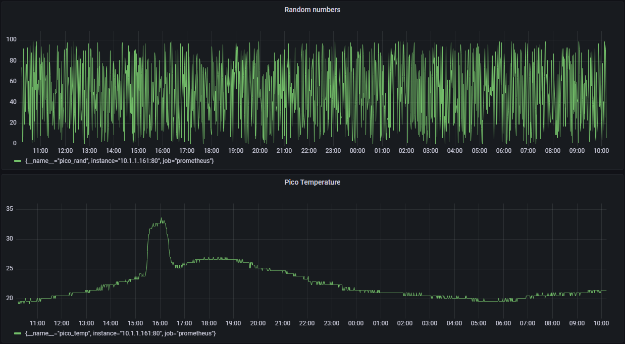
The graph above shows a 24 hour read-out of the random number and temperature metrics. The ‘blip’ that we can see around 1600 hrs is actually when the sun came through the office and passed over the Pico when it was sitting on the bench.

Make it your own

To use this code for yourself you will need to ensure that the metric you’re recording is made available in the HTML code in the while loop. Then ensure that you can replace the unique place-holder with the metric value. From there, Prometheus should do the rest.

You will have noticed that this description of how to make a measured value available to Prometheus for monitoring and display does not include a description of how to install and configure Prometheus. That’s a much longer story and I would recommend that if you don’t have an instance already installed, that you take a look at the book on installing it here.

Sending an email from a Raspberry Pi Pico W

Sending emails programmatically is a useful function for those sort of events where you have your Pico measuring something and when it needs some higher attention it sends a call for help. Kind of the Pico version of shining the bat symbol in the sky. I’m sure that there are better analogies, but that’s what I think of when I imagine a Raspberry Pi Pico sending an email.

Whatever the occasion, the Pico is up for the job.

The slightly tricky part of email.

Well… Not so much tricky, but being prepared. An email needs to originate from an email service (like Google or Outlook or ProtonMail). Our Pico isn’t quite capable enough to run an email server for us, but it can contact one that we have an account with and instruct it to send one on our behalf. That means that we need to do a little bit of research prior to setting up our code so that we have the details that are required to negotiate with our email server.

In this example we’ll use the Gmail service to send our email for us. This means that we are going to need to know details similar to the following;

• Server: smtp.gmail.com (this is hard coded into the script below)
• Sender Email: The email address that we will be sending from. I.e. Our Gmail address of (the sender).
• Sender Password: the password of the sender account. For Raspberry Pi Pico to send an email with Gmail first, we need to create an ‘App password’ using our Gmail account. An app password is a unique password generated for an app or device, as the device in this case (our Pico) will not be able to prompt for a verification code. In these cases, we can generate an app password to use instead of our regular password for accessing Gmail. We then use this password on the device. The device password is only valid for a specific device and is designed to protect the main account if the Pico gets out of control and needs to be shut down because it starts to spam people. Do a Google search for ‘create Gmail app password’ and it will guide you to the right place.
• Server port: 465 (this the port for SSL and will allow for a secure connection to the mail server)

If you’re not using Gmail you will need to determine the appropriate smtp server name for your service and the port that they use. This will vary from provider to provider and might require some googling.

We’ll also need some basics like our SSID name and username / password for connecting to the WiFi connection that will be used. Just like we needed when setting up WiFi earlier.

All this good information above can be captured in our ‘secrets.py’ file that we can keep on the Pico so that we don’t need to expose those more sensitive details in our main code. We first saw this file used in the section where we were serving a web page using the Pico. For this example it will look a little like the following (but with your secrets in the appropriate places);

secrets = {
    'ssid': '<your ssid>',
    'pw': '<your password>',
    'ip': '<the static IP address for the Pico',
    'netmask': '<the netmask for your network, but probably something like 255.25\
5.255.0>',
    'gateway': '<Your gateway address>',
    'dns': '<The DNS server you are going to use>',
    'sender_email': '<the email address of the Gmail account you will use>',
    'sender_name': '<Your sender name>',
    'sender_password': '<the App / device password that you set up in Gmail>', 
    'recipient_email': '<the email address of the recipient>' 
    }

The Code

The email function is driven by the umail module. This has been published on GitHub by shawwwn. To make use of the module we will need to download it from GitHub and then copy it over to our Pico. I found this most easily accomplished by first downloading the file to the main computer and then going File >> Open on Thonny and selecting the appropriate file. From there go File >> Save as… and select the Pico as the location to save the file (making sure to save it with the appropriate name (umail.py)).

Our code is fairly straight forward in that it imports the appropriate modules, creates the WiFi connection and then sends the email (not forgetting the secrets file) and looks like the following;

import network
import time
import umail
from secrets import secrets

# Set up Wifi
ssid = secrets['ssid']
password = secrets['pw']
rp2.country('NZ') # change to your country code

wlan = network.WLAN(network.STA_IF)

ip = secrets['ip']
netmask = secrets['netmask']
gateway = secrets['gateway']
dns = secrets['dns']

wlan.active(True) # activate the interface
if not wlan.isconnected(): # check if connected to an AP
    print('Connecting to network...')
    wlan.connect(ssid, password) # connect to an AP
    wlan.ifconfig((ip,netmask,gateway,dns))
    while not wlan.isconnected(): # wait till we are connected
        print('.', end='')
        time.sleep(0.1)
    print()
    print('Connected:', wlan.isconnected())
else:
    print("Already connected!")

# Email details
sender_email = secrets['sender_email']
sender_name = secrets['sender_name']
sender_password = secrets['sender_password']
recipient_email = secrets['recipient_email'] 
email_subject ='Test Email from Raspberry Pi Pico'

# Connect to Gmail via SSL
smtp = umail.SMTP('smtp.gmail.com', 465, ssl=True)
# Login to the email account using the senders password
smtp.login(sender_email, sender_password)
# Specify the recipient
smtp.to(recipient_email)
# Write the email header
smtp.write("From:" + sender_name + "<"+ sender_email+">\n")
smtp.write("Subject:" + email_subject + "\n")
# Write the body of the email
smtp.write("Roses are red.\n")
smtp.write("Violets are blue.\n")
smtp.write("...\n")
# Send the email
smtp.send()
# Quit the email session

Obviously the content of the body of the email can be adjusted to accept information gleaned from sensors or similar important information. Separate each line out with a newline character and we’re good to go!

Integrating a Real Time Clock (RTC) with a Raspberry Pi Pico

Just what is a RTC?

A Real Time Clock (RTC) is a crucial component for any microcontroller-based system that needs to keep track of time. Ostensibly this would then allow the system to maintain time even when the system is powered off or reset.

An RTC is a small, clock circuit that is designed to keep track of the current date and time. It typically includes a clock crystal oscillator, a battery, and a small amount of non-volatile memory for storing the time and date information.

Typically RTC’s will be separate modules that can interface with a microcontroller using a variety of communication protocols such as I2C, SPI, or UART to read and write the date and time information. The RTC provides accurate timekeeping for the microcontroller and can be used to timestamp events, trigger time-based events, and schedule tasks.

An RTC is especially useful for systems that require time-sensitive actions such as data logging, scheduling, and timing critical operations. It can also be used to implement features such as alarms, timers, and watchdogs (used to facilitate automatic correction of temporary hardware faults).

Overall, an RTC is an essential component for any microcontroller-based system that needs to keep accurate track of time, even when power is lost or the system is reset.

The RTC on a Raspberry Pi Pico

The RP2040 chip in the Raspberry Pi Pico incorporates a Real Time Clock internally. This derives an accurate time from a reference oscillator (internal by default, although an external reference is possible) and a fixed start time (which in the Pico appears to be initialised to start on the 1st of January 2021.

This is great, but there is a bit of a caveat. When the Pico is first started, without an external reference point it will default to the time being the 1st of January 2021. The worst case scenarios for this type of set up is when there is a power interruption and the time gets reset. It can be overcome in many external modules by utilising a battery backup that preserves the timing circuit, but this is not built into the Pico.

Therefore, it is useful to find a method to synchronise the Pico with an external time source to ensure that the time is accurate. This can be most easily accomplished by using a WiFi connection on the Pico W to use the Network Time Protocol to find the correct time.

From there we can use Greenwich Mean Time (GMT) (now referred to as Coordinated Universal Time or Universal Time Coordinated (UTC)) to know what time it is.

Hang on a minute I hear you say. I want to know what the time is in the country where I am running my Pico! I hear you and I acknowledge your concerns. Sadly this turns out to be way more difficult that it seems at face value. It appears that keeping track of local times is a complex job more suited to super computers and rooms full of frustrated programmers with sleeping disorders. In short, we need to learn to embrace UTC and where required to convert to our respective local times we do it as required (i.e programmatically in a script or spreadsheet. This is the only way we preserve our sanity.

The Code

The following code connects to our local WiFi network (using the secrets file to set all the appropriate network particulars (see the WiFi section for details)). From there it connects to a NTP server, pulls a time value and sets the Pico’s RTC. Then it goes about logging a timestamp every 30 seconds and flashing the on-board LED every time it writes a value to memory.

import network
import socket
import time
import struct
import machine

from secrets import secrets

NTP_DELTA = 2208988800
host = "pool.ntp.org"

rtc=machine.RTC()

def set_time():
    # Get the external time reference
    NTP_QUERY = bytearray(48)
    NTP_QUERY[0] = 0x1B
    addr = socket.getaddrinfo(host, 123)[0][-1]
    s = socket.socket(socket.AF_INET, socket.SOCK_DGRAM)
    try:
        s.settimeout(1)
        res = s.sendto(NTP_QUERY, addr)
        msg = s.recv(48)
    finally:
        s.close()

    #Set our internal time
    val = struct.unpack("!I", msg[40:44])[0]
    tm = val - NTP_DELTA    
    t = time.gmtime(tm)
    rtc.datetime((t[0],t[1],t[2],t[6]+1,t[3],t[4],t[5],0))

wlan = network.WLAN(network.STA_IF)

# Set up Wifi connection details
ssid = secrets['ssid']
password = secrets['pw']
rp2.country('NZ') # change to <your> country code
ip = secrets['ip']
netmask = secrets['netmask']
gateway = secrets['gateway']
dns = secrets['dns']

# Connect to Wifi
wlan.active(True) # activate the interface
if not wlan.isconnected(): # check if connected to an AP
    print('Connecting to network...')
    wlan.connect(ssid, password) # connect to an AP
    wlan.ifconfig((ip,netmask,gateway,dns))
    while not wlan.isconnected(): # wait till we are connected
        print('.', end='')
        time.sleep(0.1)
    print()
    print('Connected:', wlan.isconnected())
else:
    print("Already connected!")

led_onboard = machine.Pin('LED', machine.Pin.OUT)
led_onboard.value(0)

file = open("timestamps.txt", "a")

#Set our RTC
set_time()

# Log some time
while True:
    timestamp=rtc.datetime()
    timestring="%04d-%02d-%02d %02d:%02d:%02d"%(timestamp[0:3] +
                                                timestamp[4:7])
    print(timestring)
    file.write(timestring + "\n")
    file.flush()
    led_onboard.value(1)
    time.sleep(0.01)
    led_onboard.value(0)
    time.sleep(30)

For general use we would replace the data logger portion of the code to allow it to carry out whatever task we desired that included accurate time!

What gives? My Pico appears to have accurate time already!

For those who (like me) were a bit confused when not only did their Raspberry Pi Pico return accurate time while it was connected to my computer, but it returned it in accurate local time. There is a cool reason for this.

A change in the code for Thonny was introduced which allowed a small piece of code to be executed on a host computer (Windows, Mac or Linux) that will automagically find a connected Pico and then synchronise its date and time.

No MicroPython code needs be added or running on the Pico for this to work. It works by injecting a small MicroPython script, which it modifies on the fly with the host computers UTC, into the Pico over the USB serial link using the RAW REPL functionality of MicroPython! how about that.

General Pico Tips and Tricks

Universal LED Blink

As discussed in the MicroPython section of the book, the on-board LED on the original Pico corresponds with GPIO pin 25, but this was changed to be connected to one of the GPIO pins from the wireless chip (CYW43439) on the Pico W. The examples used in this book use code suitable for the Pico W and to adapt any of that code for the Pico we need to change ‘LED’ for 25 in the following code example;

from machine import Pin
led = Pin('LED', Pin.OUT)
led.value(1)

However, as responsible engineers with an eye to the foibles of uncertain hardware changes, it might be useful if we had some code that would allow us to illuminate the LED independent of which board we were using. Well good news, we can utilise the board class of functions that will allow us to determine just which type of Pico we are using and this will let us set the LED pin appropriately. The following code demonstrates this;

from machine import Pin
from board import Board
import time


BOARD_TYPE = Board().type
print("Board type: " + BOARD_TYPE)

if BOARD_TYPE == Board.BoardType.PICO_W:
    led = Pin("LED", Pin.OUT)
elif BOARD_TYPE == Board.BoardType.PICO:
    led = Pin(25, Pin.OUT)

while (True):
    led.on()
    time.sleep(.2)
    led.off()
    time.sleep(.2)

The Watchdog Timer

A WatchDog Timer (WDT) is a hardware timer that is used to detect and recover from errors in our programs or faults in their execution. Once initiated, a watchdog timer is constantly counting down and when (or if) it reaches zero, it reboots our device. The only thing that stops the timer reaching zero is periodic resetting of the timer back to its starting position. We place lines in our code at strategic points that perform this reset, so that under normal operation the timer should never reach zero. These resets are referred to as ‘patting the dog’, ‘feeding the dog’ or cruelly, ‘kicking the dog’ (not happy about that one).

While we aren’t going to purposely design our software to freeze, strange things can happen (cosmic rays - really!) and it is often practical to prepare for the unexpected. Conversely, you might notice that your device hangs for no apparent reason after long periods. Weird stuff does happen. When it’s more important that the system keeps functioning than it is to troubleshoot the problem, a watchdog timer could be your friend.

In the Raspberry Pi Pico or more precisely the RP2040, the watchdog has a 24-bit counter that decrements from a user defined value. The maximum time between resetting the watchdog counter is approximately 8.3 seconds before it reaches zero and reboots our device.

In a very simple code example from the MicroPython documentation we can see the watchdog timer library loaded, the timer is enabled with a time of 2000 milliseconds (2 seconds) and then the watchdog is fed.

from machine import WDT
wdt = WDT(timeout=2000)  # enable it with a timeout of 2s
wdt.feed()

In our code we would set our timer appropriate for the occasion and place the feeding statements in strategic places so that under normal circumstances, there shouldn’t be a situation where it would run down for more than the specified amount of time before being fed again.

Logging to Help with Troubleshooting

Alrighty… Let’s get the obvious part of the discussion on this topic out of the way…

There are a wide range of possible mechanisms for troubleshooting depending on the skill level of the practitioner, the complexity of the code and the capabilities of the platform. In short, you will ultimately fall to using the techniques that work for you the best depending on your circumstances.

I am capturing the description of this method, not because I think it is the best or even if I think that it’s advisable. It suited me for a task and so I believed that it might suit me again at some time in the future. Therefore I thought I should write this down so that I don’t forget what the code does, and what better place to write it down than in a book :-).

This particular piece of code is written to capture notes as our Micropython code executes and to write those notes into a log file so that we can examine them at a later date. The particular occasion I needed something like this was when I had a Pico that would run for many days and would then fail. I couldn’t determine why it was failing, and so I decided that a piece of code that would write lines to a file so that I could see when and where the failure occurred would be a good start.

Therefore, the way this piece of code would be used is if we place the initial set-up and function definition at the start of the program we are troubleshooting and then we place the small note capturing code at various places where we want to know that the program has gotten to or looking at values that we want to check.

It captures the time that the event is written, the size of the log file and the message that we want to pass to it. This message can be text and / or values.

Enough talk, this is what it looks like;

import os
from machine import RTC

rtc = RTC()
rtc.datetime()

#Check to see if file present and create if necessary
try:
    os.stat('/log.dat')
    print("File Exists")
except:
    print("File Missing")
    f = open("log.dat", "w")
    f.close()
    
def log(loginfo:str):
    # Format the timestamp
    timestamp=rtc.datetime()
    timestring="%04d-%02d-%02d %02d:%02d:%02d"%(timestamp[0:3] +
                                                timestamp[4:7])
    # Check the file size
    filestats = os.stat('/log.dat')
    filesize = filestats[6]

    if(filesize<200000):
        try:
            log = timestring +" "+ str(filesize) +" "+ loginfo +"\n"
            print(log)
            with open("log.dat", "at") as f:
                f.write(log)
        except:
            print("Problem saving file")

# sample usage
val = 456
text = "some information"
combo = text + " " + str(val)
log(combo)

To make life easier for future me (and hopefully you) here’s the description of some of the parts.

We import the os module and RTC from machine

import os
from machine import RTC

rtc = RTC()
rtc.datetime()

This is so that we can us the os module to determine the size of the file we are generating and to make sure that we don’t write so large a file that it overwhelms our available storage.

RTC is used to generate a timestamp so that we know when an event occurs. Of course, if we don’t set the time initially, we are going to be left with a time stamp that starts at 2021-01-01 00:00:00. We could connect to NTP time first if we had a network connection, but that’s not always going to be available. This way we will at least have a feel for how our comments are being captured relative to each other and the time that the program started. There are several different time modules that we could use to do this. time, utime, and possibly others. Each has some slight differences in terms of the start of the timestamp or similar, and I fell on RTC. It does the job.

If the file that we’re going to use for capturing our information doesn’t exist, we need to create it.

#Check to see if file present and create if necessary
try:
    os.stat('/log.dat')
    print("File Exists")
except:
    print("File Missing")
    f = open("log.dat", "w")
    f.close()

The first use of the open command to append information to a file will create the file if it doesn’t exist, but we will want to check the size of the file before we write anything to it, so this small piece of code checks for its existence and if it isn’t there creates it.

Then we get into the function definition.

We find the time and format it as a string in a nice tidy format. For those of you who are writing your dates in a dd/mm/yyyy format, using the alternative of yyyy/mm/dd makes it easier to sort.

    # Format the timestamp
    timestamp=rtc.datetime()
    timestring="%04d-%02d-%02d %02d:%02d:%02d"%(timestamp[0:3] +
                                                timestamp[4:7])

We can then check out the file size;

    # Check the file size
    filestats = os.stat('/log.dat')
    filesize = filestats[6]

The os.stat call responds with a range of different metrics (not all of which are applicable for every platform). The one we want is accessed as [6] in the array.

After checking to make sure that our file hasn’t grown too large we combine the time, the size of the file and the information that we want to note specifically (this comes from then individual calls to the function in the program).

            log = timestring +" "+ str(filesize) +" "+ loginfo +"\n"
            print(log)
            with open("log.dat", "at") as f:
                f.write(log)

We also add a newline "\n" in to break the lines up.

The final block of the code is the piece that we would put in a range of places in our program to capture information.

# sample usage
val = 456
text = "some information"
combo = text + " " + str(val)
log(combo)

This is obviously just a sample, but we have a value val that could be any number used in the program and a comment some information that again could be something that acts as a reference for that portion of the code that we’re wanting to know something about. For example, it could be when the program starts and then when the device connects to the network, and then if it strikes an error in reading a value from a sensor.